LGCPs - Spatial covariates • inlabru

Set things up

library(INLA)
library(inlabru)
library(fmesher)
library(RColorBrewer)
library(ggplot2)
library(patchwork)
# Activate DIC output
bru_options_set(control.compute = list(dic = TRUE, waic = TRUE))

Introduction

We are going to fit spatial models to the gorilla data, using factor and continuous explanatory variables in this practical. We will fit one using the factor variable vegetation, the other using the continuous covariate elevation

(Jump to the bottom of the practical if you want to start gently with a 1D example!)

Get the data

data(gorillas_sf, package = "inlabru")

This dataset is a list (see help(gorillas_sf) for details. Extract the objects you need from the list, for convenience:

nests <- gorillas_sf$nests
mesh <- gorillas_sf$mesh
boundary <- gorillas_sf$boundary
gcov <- gorillas_sf_gcov()
#> Loading required namespace: terra

Factor covariates

Look at the vegetation type, nests and boundary:

ggplot() +
  gg(gcov$vegetation) +
  gg(boundary, alpha = 0.2) +
  gg(nests, color = "white", cex = 0.5)

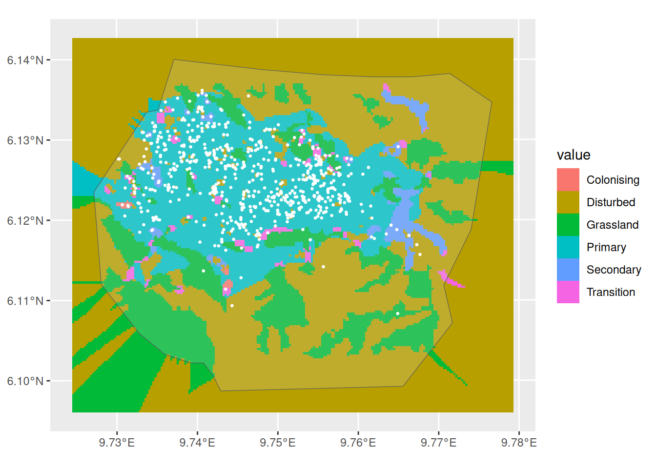
Or, with the mesh:

ggplot() +
  gg(gcov$vegetation) +
  gg(mesh) +
  gg(boundary, alpha = 0.2) +
  gg(nests, color = "white", cex = 0.5)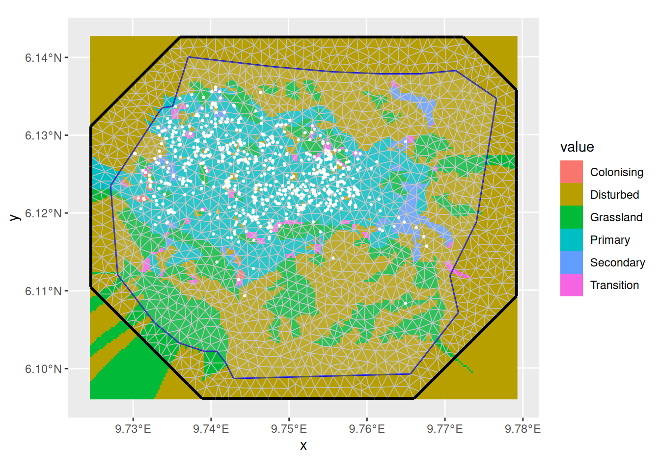

A model with vegetation type only

It seems that vegetation type might be a good predictor because nearly all the nests fall in vegetation type Primary. So we construct a model with vegetation type as a fixed effect. To do this, we need to tell ‘lgcp’ how to find the vegetation type at any point in space, and we do this by creating model components with a fixed effect that we call vegetation (we could call it anything), as follows:

comp_veg <- geometry ~ vegetation(gcov$vegetation, model = "factor_full") - 1

Notes: * We need to tell ‘lgcp’ that this is a factor fixed effect, which we do with model="factor_full", giving one coefficient for each factor level. * We need to be careful about overparameterisation when using factors. Unlike regression models like ‘lm()’, ‘glm()’ or ‘gam()’, ‘lgcp()’, inlabru does not automatically remove the first level and absorb it into an intercept. Instead, we can either use model="factor_full" without an intercept, or model="factor_contrast", which does remove the first level.

comp_veg_alt <-
  geometry ~ vegetation(gcov$vegetation, model = "factor_contrast") +
  Intercept(1)

To enable group.cv calculations, we need to split the domain into spatial regions, and compute the association of each observed point to these subregions.

cvpart <- cv_hex(boundary, cellsize = 0.4, n_group = 3)

ggplot() +
  gg(cvpart, aes(fill = group), alpha = 0.5) +
  gg(boundary, alpha = 0) +
  gg(nests, color = "white", cex = 0.5)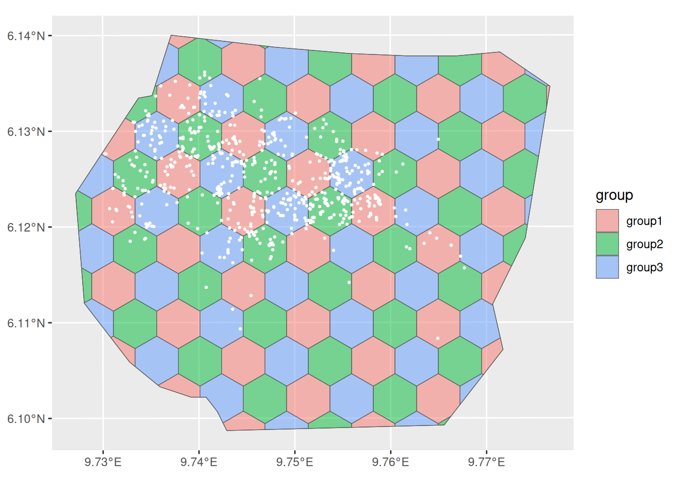


cvpart$block_ID <- seq_len(nrow(cvpart))
cvpart$group <- NULL
a <- sf::st_intersects(nests, cvpart)
if (any(lengths(a) != 1)) {
  stop("Point in none or multiple polygons")
}
nests$.block <- unlist(a)

Fit the model as usual, and increasing the integration scheme resolution to better match the covariate:

mesh_int <- fm_subdivide(mesh, 2)
fit_veg <- lgcp(
  comp_veg,
  nests,
  samplers = cvpart,
  domain = list(geometry = mesh_int),
  control.gcpo = list(enable = FALSE, type.cv = "joint", num.level.sets = 2),
  options = list(bru_verbose = 0)
)
#  options = list(control.compute = list(control.gcpo = list(enable = TRUE))))

Predict the intensity, and plot the median intensity surface. (In older versions, predicting takes some time because we did not have vegetation values outside the mesh so ‘inlabru’ needed to predict these first. Since v2.0.0, the vegetation has been pre-extended.)

The predict function of inlabru takes into its data argument an sf object or other object supported by the predictor evaluation code (for non-geographical data, typically a data.frame). We can use the inlabru function pixels to generate an sf object with points only within the boundary, using its mask argument, as shown below.

pred.df <- fm_pixels(mesh, mask = boundary)
intensity_veg <- predict(fit_veg, pred.df, ~ exp(vegetation))

# gg() with sf points and geom = "tile" plots a raster
ggplot() +
  gg(intensity_veg, geom = "tile") +
  gg(boundary, alpha = 0, lwd = 2) +
  gg(nests, color = "DarkGreen")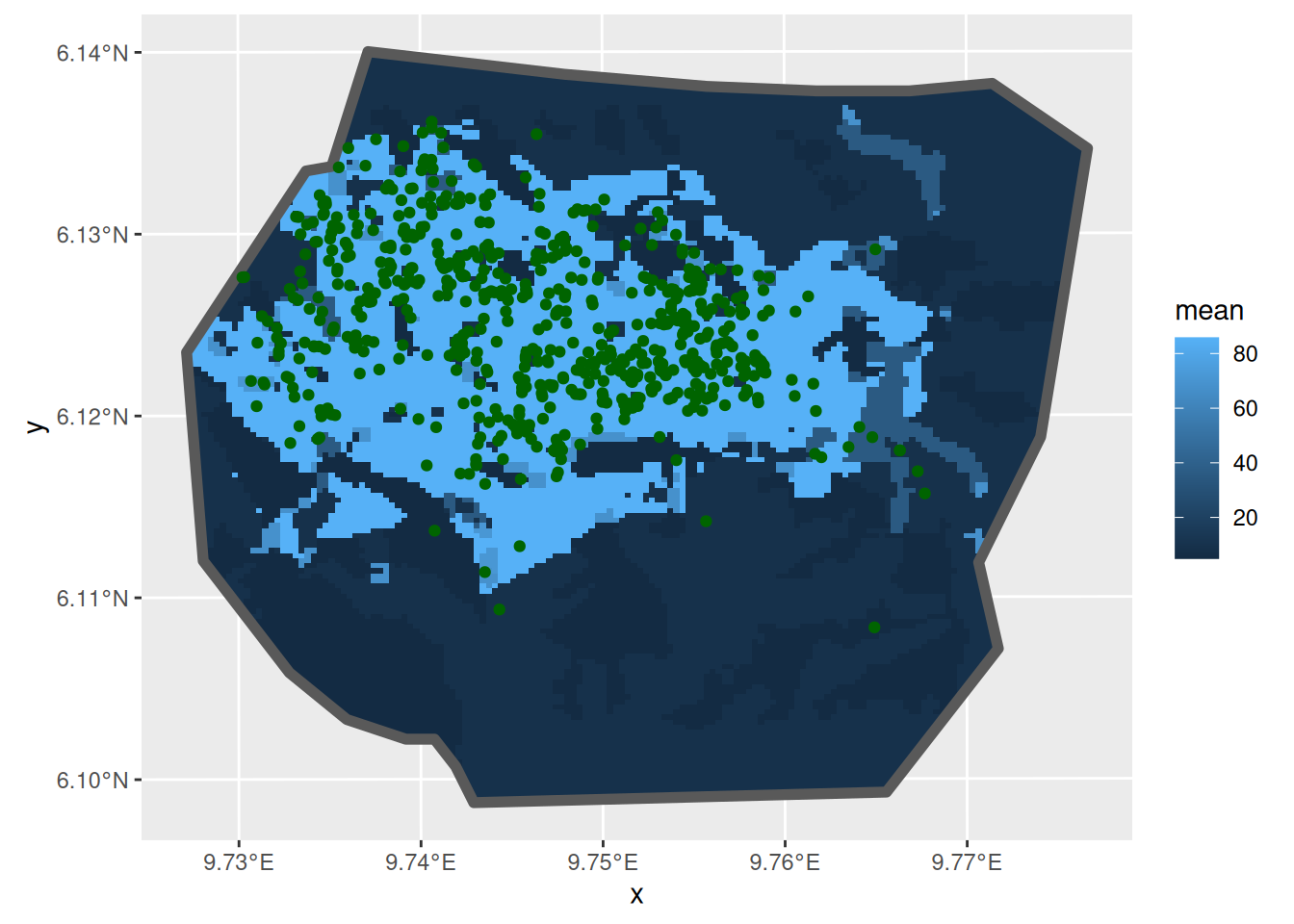

Not surprisingly, given that most nests are in Primary vegetation, the high density is in this vegetation. But there are substantial patches of predicted high density that have no nests, and some areas of predicted low density that have nests. What about the estimated abundance (there are really 647 nests there):

ips <- fm_int(list(geometry = mesh_int), boundary)
Lambda_veg <- predict(fit_veg, ips, ~ sum(weight * exp(vegetation)))
Lambda_veg
#>       mean       sd   q0.025     q0.5   q0.975   median mean.mc_std_err
#> 1 650.4694 24.91121 603.4231 651.2843 700.6565 651.2843        2.878215
#>   sd.mc_std_err
#> 1      1.935467

Continuous limit of WAIC

IC <- lgcp_IC(
  fit_veg,
  data = nests,
  predictor = vegetation,
  domain = list(geometry = mesh_int),
  samplers = cvpart
)
knitr::kable(IC)

Criterion	Method	lppd	p_eff	IC	lppd.std_err	p_eff.std_err	IC.std_err
DIC	Limit	1998.468	6.258784	-3984.417	0.5730897	0.3399997	1.8261788
DIC	INLA	1978.534	5.879493	-3945.309	NA	NA	NA
DIC_adjusted	INLA	1998.408	5.879493	-3985.057	NA	NA	NA
WAIC	Limit	1998.468	6.031679	-3984.872	0.5730897	0.0224830	1.1911453
WAIC	Blockwise	2121.480	11.146392	-4220.667	0.1077651	0.0836815	0.3828932
WAIC	INLA	1978.842	6.502853	-3944.678	NA	NA	NA
WAIC_adjusted	INLA	1998.716	6.502853	-3984.425	NA	NA	NA

Cross validation with NA setting

fit_veg2_prep <- bru_set_missing(
  fit_veg,
  keep = list(-which(
    as_bru_obs_list(fit_veg)[[1]]$response_data$BRU_block == 8L
  ))
)
fit_veg2 <- bru_rerun(fit_veg2_prep)

A model with vegetation type and a SPDE type smoother

Lets try to explain the pattern in nest distribution that is not captured by the vegetation covariate, using an SPDE:

pcmatern <- inla.spde2.pcmatern(mesh,
  prior.sigma = c(1, 0.01),
  prior.range = c(0.1, 0.01)
)

comp_veg_field <- geometry ~
  -1 +
  vegetation(gcov$vegetation, model = "factor_full") +
  field(geometry, model = pcmatern)

fit_veg_field <- lgcp(comp_veg_field,
  nests,
  samplers = boundary,
  domain = list(geometry = mesh_int)
)

And plot the posterior median intensity surface

intensity_veg_field <-
  predict(
    fit_veg_field,
    pred.df,
    ~ exp(field + vegetation),
    n.samples = 1000
  )

ggplot() +
  gg(intensity_veg_field, aes(fill = q0.5), geom = "tile") +
  gg(boundary, alpha = 0, lwd = 2) +
  gg(nests)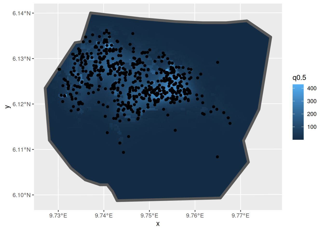

… and the expected integrated intensity (mean of abundance)

Lambda_veg_field <- predict(
  fit_veg_field,
  fm_int(mesh_int, boundary),
  ~ sum(weight * exp(field + vegetation))
)
Lambda_veg_field
#>       mean       sd   q0.025    q0.5   q0.975  median mean.mc_std_err
#> 1 692.5571 27.19803 636.0883 691.236 740.7869 691.236        3.105301
#>   sd.mc_std_err
#> 1      1.927493

Look at the contributions to the linear predictor from the SPDE and from vegetation:

lp_veg_field <- predict(fit_veg_field, pred.df, ~ list(
  smooth_veg = field + vegetation,
  smooth = field,
  veg = vegetation
))

The function scale_fill_gradientn sets the scale for the plot legend. Here we set it to span the range of the three linear predictor components being plotted (medians are plotted by default).

lprange <- range(
  lp_veg_field$smooth_veg$median,
  lp_veg_field$smooth$median,
  lp_veg_field$veg$median
)
csc <- scale_fill_gradientn(colours = brewer.pal(9, "YlOrRd"), limits = lprange)

plot.lp_veg_field <- ggplot() +
  gg(lp_veg_field$smooth_veg, geom = "tile") +
  csc +
  gg(boundary, alpha = 0) +
  ggtitle("field + vegetation")

plot.lp_veg_field.spde <- ggplot() +
  gg(lp_veg_field$smooth, geom = "tile") +
  csc +
  gg(boundary, alpha = 0) +
  ggtitle("field")

plot.lp_veg_field.veg <- ggplot() +
  gg(lp_veg_field$veg, geom = "tile") +
  csc +
  gg(boundary, alpha = 0) +
  ggtitle("vegetation")

(plot.lp_veg_field + plot.lp_veg_field.spde + plot.lp_veg_field.veg) +
  plot_layout(ncol = 3, guides = "collect") &
  guides(fill = guide_legend("value")) &
  theme(legend.position = "right")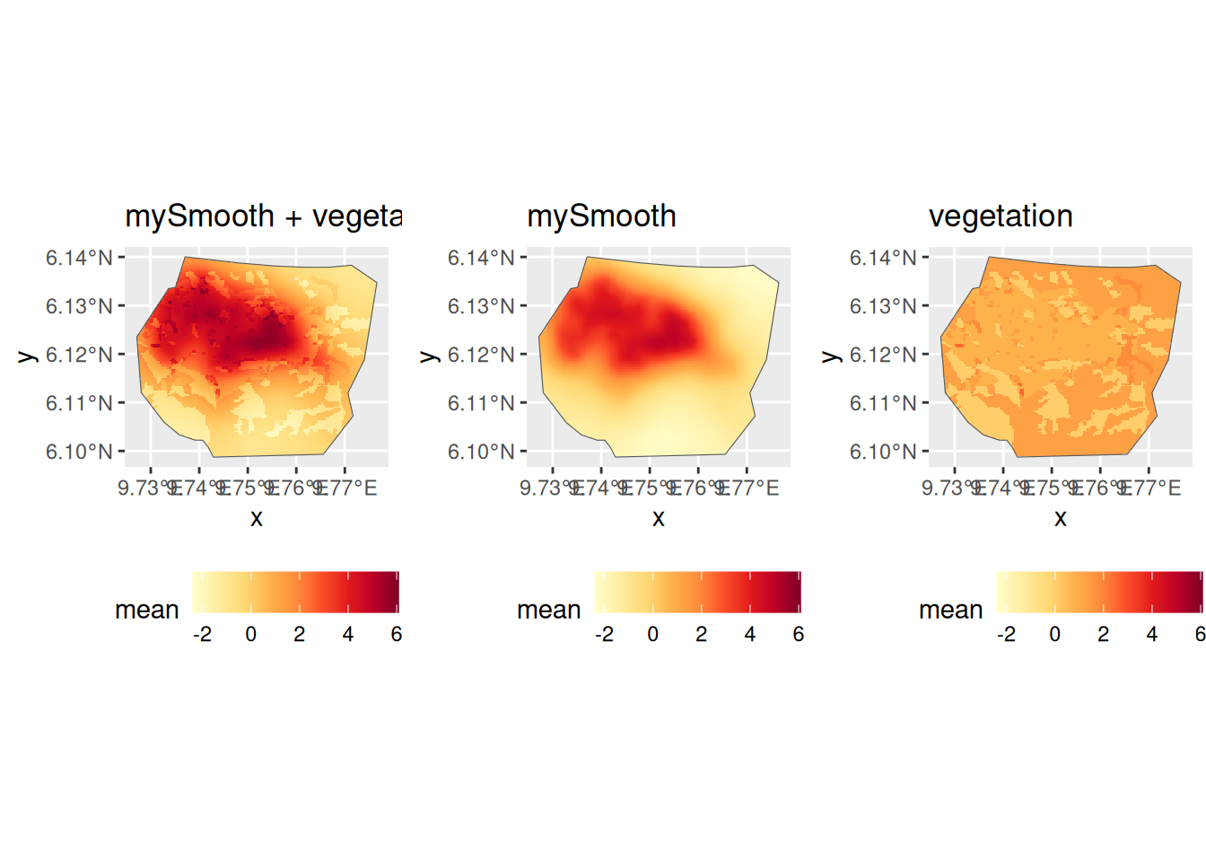

A model with SPDE only

Do we need vegetation at all? Fit a model with only an SPDE + Intercept, and choose between models on the basis of DIC, using deltaIC().

comp_field <- geometry ~ field(geometry, model = pcmatern) + Intercept(1)
fit_field <- lgcp(comp_field,
  data = nests,
  samplers = boundary,
  domain = list(geometry = mesh_int),
  options = list(control.compute(dic = TRUE))
)

intensity_field <- predict(fit_field, pred.df, ~ exp(field + Intercept))

ggplot() +
  gg(intensity_field, geom = "tile") +
  gg(boundary, alpha = 0) +
  gg(nests)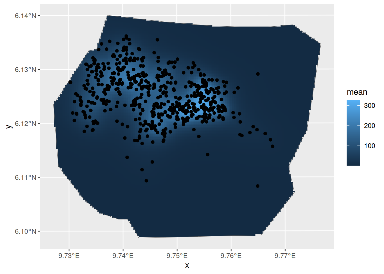

Lambda_field <- predict(
  fit_field,
  fm_int(mesh_int, boundary),
  ~ sum(weight * exp(field + Intercept))
)
Lambda_field
#>       mean       sd   q0.025    q0.5   q0.975  median mean.mc_std_err
#> 1 692.2893 28.13998 638.3449 692.695 741.8783 692.695        3.192524
#>   sd.mc_std_err
#> 1      1.892633

knitr::kable(deltaIC(fit_veg, fit_veg_field, fit_field, criterion = c("DIC")))

Model	DIC	Delta.DIC
fit_veg_field	-4897.277	0.0000
fit_field	-4876.514	20.7627
fit_veg	-3945.309	951.9677

New experimental definitions:

IC_veg <- lgcp_IC(
  fit_veg,
  data = nests,
  predictor = vegetation,
  domain = list(geometry = mesh_int),
  samplers = cvpart
)
IC_veg_field <- lgcp_IC(
  fit_veg_field,
  data = nests,
  predictor = vegetation + field,
  domain = list(geometry = mesh_int),
  samplers = cvpart
)
IC_field <- lgcp_IC(
  fit_field,
  data = nests,
  predictor = field + Intercept,
  domain = list(geometry = mesh_int),
  samplers = cvpart
)
IC_data <- rbind(
  cbind(IC_veg, Model = "veg"),
  cbind(IC_veg_field, Model = "veg + field"),
  cbind(IC_field, Model = "field")
)
knitr::kable(IC_data |>
  dplyr::arrange(Criterion, Method, Model))

Criterion	Method	lppd	p_eff	IC	lppd.std_err	p_eff.std_err	IC.std_err	Model
DIC	INLA	2547.124	108.867079	-4876.514	NA	NA	NA	field
DIC	INLA	1978.534	5.879493	-3945.309	NA	NA	NA	veg
DIC	INLA	2558.934	110.295101	-4897.277	NA	NA	NA	veg + field
DIC	Limit	2555.321	286.456318	-4537.729	0.6967043	9.8573881	21.1081849	field
DIC	Limit	1998.468	6.163183	-3984.609	0.5962845	0.3196793	1.8319275	veg
DIC	Limit	2567.887	301.864896	-4532.045	0.7080791	16.1083682	33.6328946	veg + field
DIC_adjusted	INLA	2566.998	108.867079	-4916.262	NA	NA	NA	field
DIC_adjusted	INLA	1998.408	5.879493	-3985.057	NA	NA	NA	veg
DIC_adjusted	INLA	2578.807	110.295101	-4937.024	NA	NA	NA	veg + field
WAIC	Blockwise	2409.438	34.175988	-4750.524	0.0859464	0.3295766	0.8310461	field
WAIC	Blockwise	2122.192	11.572380	-4221.239	0.0900241	0.0844449	0.3489380	veg
WAIC	Blockwise	2410.052	34.628098	-4750.849	0.0849694	0.6919897	1.5539182	veg + field
WAIC	INLA	2549.955	115.855886	-4868.199	NA	NA	NA	field
WAIC	INLA	1978.842	6.502853	-3944.678	NA	NA	NA	veg
WAIC	INLA	2562.992	120.025066	-4885.933	NA	NA	NA	veg + field
WAIC	Limit	2555.321	86.147384	-4938.347	0.6967043	0.1412003	1.6758093	field
WAIC	Limit	1998.468	6.038233	-3984.859	0.5962845	0.0238211	1.2402112	veg
WAIC	Limit	2567.887	88.506776	-4958.761	0.7080791	0.1445583	1.7052749	veg + field
WAIC_adjusted	INLA	2569.829	115.855886	-4907.946	NA	NA	NA	field
WAIC_adjusted	INLA	1998.716	6.502853	-3984.425	NA	NA	NA	veg
WAIC_adjusted	INLA	2582.865	120.025066	-4925.681	NA	NA	NA	veg + field

CV and SPDE parameters for Model 2

We are going with Model fit_veg_field. Lets look at the spatial distribution of the coefficient of variation

ggplot() +
  gg(intensity_veg_field, aes(fill = sd / mean), geom = "tile") +
  gg(boundary, alpha = 0) +
  gg(nests)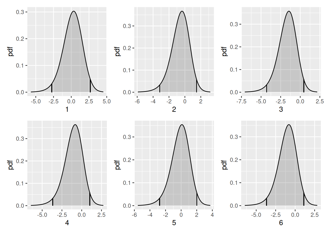

Plot the vegetation “fixed effect” posteriors. First get their names - from $marginals.random$vegetation of the fitted object, which contains the fixed effect marginal distribution data

flist <- vector("list", NROW(fit_veg_field$summary.random$vegetation))
for (i in seq_along(flist)) {
  flist[[i]] <- plot(fit_veg_field, "vegetation", index = i)
  flist_combined <- if (i == 1) flist[[i]] else flist_combined + flist[[i]]
}
flist_combined +
  plot_layout(ncol = 3, guides = "collect")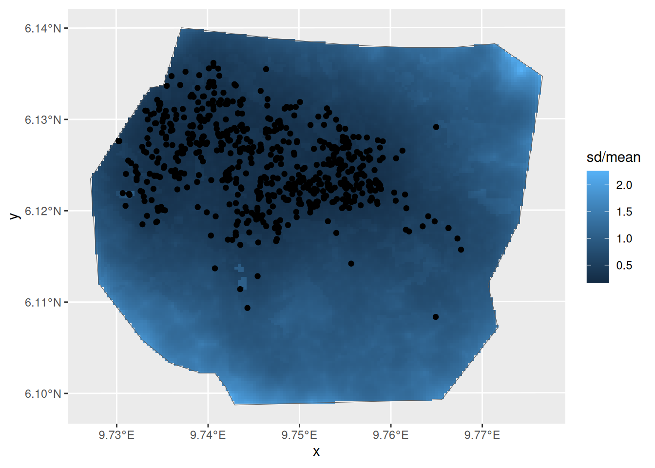

Use spde.posterior( ) to obtain and then plot the SPDE parameter posteriors and the Matern correlation and covariance functions for this model.

spde.range <- spde.posterior(fit_veg_field, "field", what = "range")
spde.logvar <- spde.posterior(fit_veg_field, "field", what = "log.variance")
range.plot <- plot(spde.range)
var.plot <- plot(spde.logvar)
(range.plot / var.plot)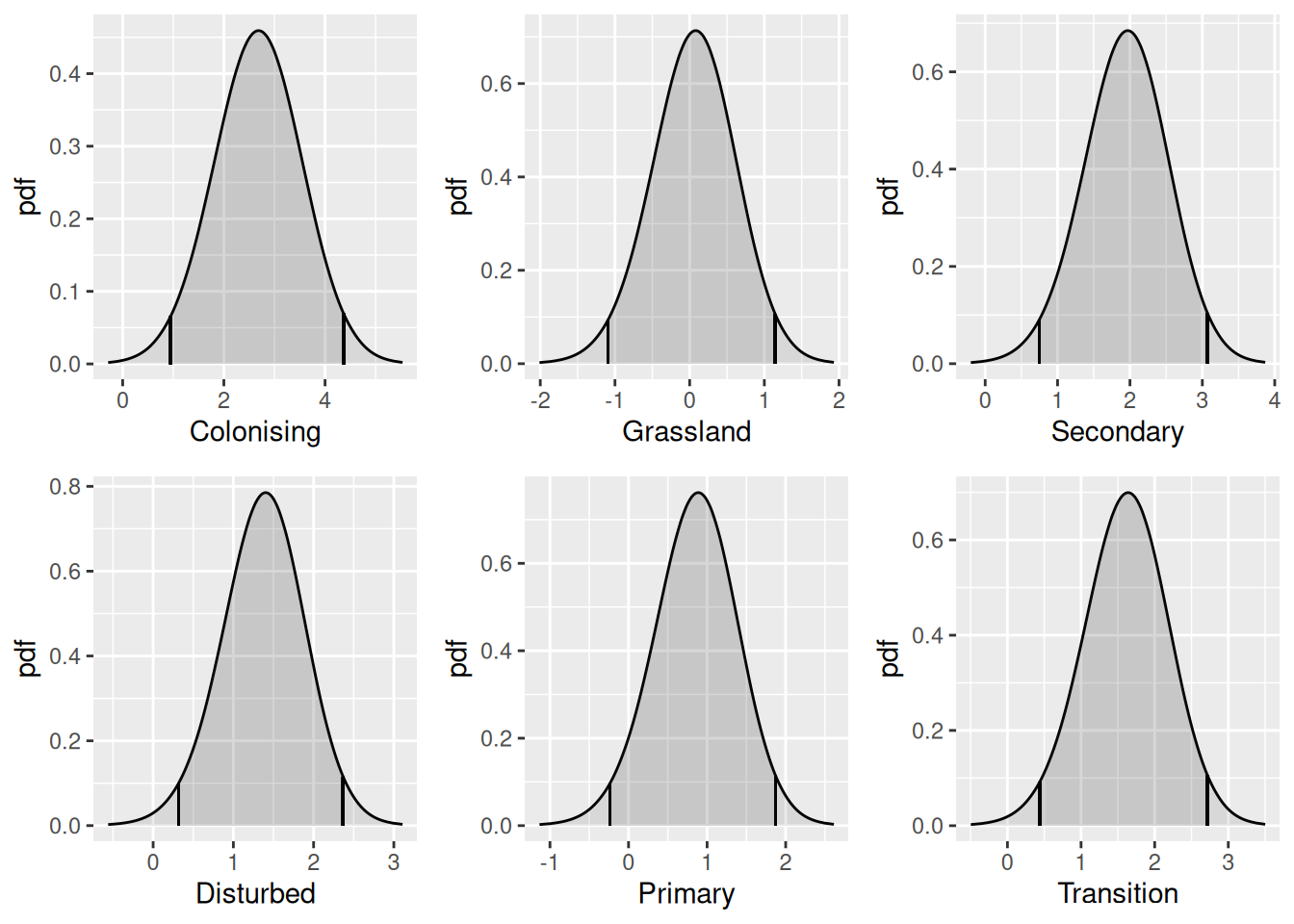


corplot <-
  plot(spde.posterior(fit_veg_field, "field", what = "matern.correlation"))
covplot <-
  plot(spde.posterior(fit_veg_field, "field", what = "matern.covariance"))
(covplot / corplot)

Continuous covariates

Now lets try a model with elevation as a (continuous) explanatory variable. (First centre elevations for more stable fitting.)

elev <- gcov$elevation
elev <- elev - mean(terra::values(elev), na.rm = TRUE)

ggplot() +
  gg(elev, geom = "tile") +
  gg(boundary, alpha = 0)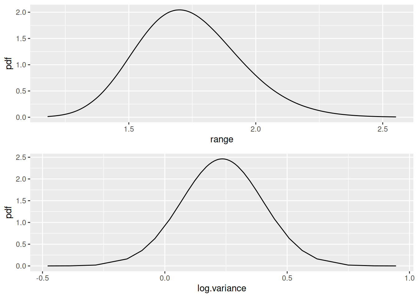

The elevation variable here is of class ‘SpatRaster’, that can be handled in the same way as the vegetation covariate, with automatic evaluation via an eval_spatial() method. However, since in some cases data may be stored differently, other methods are needed to access the stored values, or there’s some post-processing to be done. In such cases, we can define a function that knows how to evaluate the covariate at arbitrary points in the survey region, and call that function in the component definition. The method eval_spatial() is the method that handles this automatically, and supports terra SpatRaster and sf geometry points objects, and mismatching coordinate systems as well. In the following evaluator example function, we only add infilling of missing values as a post-processing step.

# Note: this method is usually not needed; the automatic invocation of
# `eval_spatial()` method by the component input evaluator is usually
# sufficient.
f.elev <- function(where) {
  # Extract the values
  v <- eval_spatial(elev, where, layer = "elevation")
  # Fill in missing values; this example would work for
  # SpatialPixelsDataFrame data
  # if (anyNA(v)) {
  #   v <- bru_fill_missing(elev, where, v)
  # }
  v
}

For brevity we are not going to consider models with elevation only, with elevation and a SPDE, and with SPDE only. We will just fit one with elevation and SPDE. We create our model to pass to lgcp thus:

matern <- inla.spde2.pcmatern(mesh,
  prior.sigma = c(1, 0.01),
  prior.range = c(0.1, 0.01)
)

comp_elev_field <- geometry ~ elev(f.elev(.data.), model = "linear") +
  field(geometry, model = matern) + Intercept(1)

Note how the elevation effect is defined. We could alternatively use the terra grid object directly (causing inlabru to automatically call eval_spatial()), like in the vegetation case: we specified it like

elev(elev, model = "factor_full")

whereas with the special function method we specify the covariate like this:

elev(f.elev(.data.), model = "linear")

Most applications can use the automatic method, and the special function method is included only as an example of how to handle more complex cases.

We also now include an intercept term in the model.

The model is fitted in the usual way:

fit_elev_field <- lgcp(comp_elev_field, nests,
  samplers = boundary,
  domain = list(geometry = mesh_int)
)

Summary and model selection

summary(fit_elev_field)
#> inlabru version: 2.14.1.9003 
#> INLA version: 26.05.10 
#> Latent components:
#> elev: main = linear(f.elev(.data.))
#> field: main = spde(geometry)
#> Intercept: main = linear(1)
#> Observation models:
#>   Model tag: <No tag>
#>     Family: 'cp'
#>     Data class: 'sf', 'tbl_df', 'tbl', 'data.frame'
#>     Response class: 'numeric'
#>     Predictor: geometry ~ elev + field + Intercept
#>     Additive/Linear/Rowwise: TRUE/TRUE/TRUE
#>     Used components: effect[elev, field, Intercept], latent[] 
#> Time used:
#>     Pre = 0.31, Running = 3.06, Post = 0.168, Total = 3.54 
#> Fixed effects:
#>             mean    sd 0.025quant 0.5quant 0.975quant   mode kld
#> elev       0.003 0.002      0.000    0.003      0.006  0.003   0
#> Intercept -0.609 1.024     -2.877   -0.530      1.181 -0.382   0
#> 
#> Random effects:
#>   Name     Model
#>     field SPDE2 model
#> 
#> Model hyperparameters:
#>                 mean    sd 0.025quant 0.5quant 0.975quant mode
#> Range for field 1.85 0.371       1.25     1.81       2.70 1.72
#> Stdev for field 2.22 0.329       1.66     2.19       2.95 2.13
#> 
#> Deviance Information Criterion (DIC) ...............: -4877.04
#> Deviance Information Criterion (DIC, saturated) ....: 320147.32
#> Effective number of parameters .....................: 111.41
#> 
#> Watanabe-Akaike information criterion (WAIC) ...: -4868.25
#> Effective number of parameters .................: 118.78
#> 
#> Marginal log-Likelihood:  2370.48 
#>  is computed 
#> Posterior summaries for the linear predictor and the fitted values are computed
#> (Posterior marginals needs also 'control.compute=list(return.marginals.predictor=TRUE)')
deltaIC(fit_veg, fit_veg_field, fit_field, fit_elev_field)
#>            Model       DIC Delta.DIC
#> 1  fit_veg_field -4897.277   0.00000
#> 2 fit_elev_field -4877.038  20.23912
#> 3      fit_field -4876.514  20.76270
#> 4        fit_veg -3945.309 951.96772

New definitions:

IC_elev_field <- lgcp_IC(
  fit_elev_field,
  data = nests,
  predictor = elev + field + Intercept,
  domain = list(geometry = mesh_int),
  samplers = cvpart
)
IC_data <- rbind(IC_data, cbind(IC_elev_field, Model = "elev + field"))
knitr::kable(IC_data |> dplyr::arrange(Criterion, Method, Model))

Criterion	Method	lppd	p_eff	IC	lppd.std_err	p_eff.std_err	IC.std_err	Model
DIC	INLA	2549.924	111.405397	-4877.038	NA	NA	NA	elev + field
DIC	INLA	2547.124	108.867079	-4876.514	NA	NA	NA	field
DIC	INLA	1978.534	5.879493	-3945.309	NA	NA	NA	veg
DIC	INLA	2558.934	110.295101	-4897.277	NA	NA	NA	veg + field
DIC	Limit	2558.195	297.088294	-4522.214	0.7198450	9.5472391	20.5341681	elev + field
DIC	Limit	2555.321	286.456318	-4537.729	0.6967043	9.8573881	21.1081849	field
DIC	Limit	1998.468	6.163183	-3984.609	0.5962845	0.3196793	1.8319275	veg
DIC	Limit	2567.887	301.864896	-4532.045	0.7080791	16.1083682	33.6328946	veg + field
DIC_adjusted	INLA	2569.798	111.405397	-4916.785	NA	NA	NA	elev + field
DIC_adjusted	INLA	2566.998	108.867079	-4916.262	NA	NA	NA	field
DIC_adjusted	INLA	1998.408	5.879493	-3985.057	NA	NA	NA	veg
DIC_adjusted	INLA	2578.807	110.295101	-4937.024	NA	NA	NA	veg + field
WAIC	Blockwise	2409.458	34.508089	-4749.900	0.0860050	0.3398912	0.8517925	elev + field
WAIC	Blockwise	2409.438	34.175988	-4750.524	0.0859464	0.3295766	0.8310461	field
WAIC	Blockwise	2122.192	11.572380	-4221.239	0.0900241	0.0844449	0.3489380	veg
WAIC	Blockwise	2410.052	34.628098	-4750.849	0.0849694	0.6919897	1.5539182	veg + field
WAIC	INLA	2552.901	118.775594	-4868.250	NA	NA	NA	elev + field
WAIC	INLA	2549.955	115.855886	-4868.199	NA	NA	NA	field
WAIC	INLA	1978.842	6.502853	-3944.678	NA	NA	NA	veg
WAIC	INLA	2562.992	120.025066	-4885.933	NA	NA	NA	veg + field
WAIC	Limit	2558.195	88.785237	-4938.820	0.7198450	0.1444085	1.7285070	elev + field
WAIC	Limit	2555.321	86.147384	-4938.347	0.6967043	0.1412003	1.6758093	field
WAIC	Limit	1998.468	6.038233	-3984.859	0.5962845	0.0238211	1.2402112	veg
WAIC	Limit	2567.887	88.506776	-4958.761	0.7080791	0.1445583	1.7052749	veg + field
WAIC_adjusted	INLA	2572.774	118.775594	-4907.998	NA	NA	NA	elev + field
WAIC_adjusted	INLA	2569.829	115.855886	-4907.946	NA	NA	NA	field
WAIC_adjusted	INLA	1998.716	6.502853	-3984.425	NA	NA	NA	veg
WAIC_adjusted	INLA	2582.865	120.025066	-4925.681	NA	NA	NA	veg + field

knitr::kable(
  IC_data |>
    delta_IC() |>
    dplyr::select(
      Method, Criterion, lppd, p_eff, IC, Delta_IC, IC.std_err, Model
    )
)

Method	Criterion	lppd	p_eff	IC	Delta_IC	IC.std_err	Model
INLA	DIC	2558.934	110.295101	-4897.277	0.0000000	NA	veg + field
INLA	DIC	2549.924	111.405397	-4877.038	20.2391166	NA	elev + field
INLA	DIC	2547.124	108.867079	-4876.514	20.7627001	NA	field
INLA	DIC	1978.534	5.879493	-3945.309	951.9677219	NA	veg
Limit	DIC	2555.321	286.456318	-4537.729	0.0000000	21.1081849	field
Limit	DIC	2567.887	301.864896	-4532.045	5.6838540	33.6328946	veg + field
Limit	DIC	2558.195	297.088294	-4522.214	15.5150941	20.5341681	elev + field
Limit	DIC	1998.468	6.163183	-3984.609	553.1200131	1.8319275	veg
INLA	DIC_adjusted	2578.807	110.295101	-4937.024	0.0000000	NA	veg + field
INLA	DIC_adjusted	2569.798	111.405397	-4916.785	20.2391166	NA	elev + field
INLA	DIC_adjusted	2566.998	108.867079	-4916.262	20.7627001	NA	field
INLA	DIC_adjusted	1998.408	5.879493	-3985.057	951.9677219	NA	veg
Blockwise	WAIC	2410.052	34.628098	-4750.849	0.0000000	1.5539182	veg + field
Blockwise	WAIC	2409.438	34.175988	-4750.524	0.3241627	0.8310461	field
Blockwise	WAIC	2409.458	34.508089	-4749.900	0.9489467	0.8517925	elev + field
Blockwise	WAIC	2122.192	11.572380	-4221.239	529.6094827	0.3489380	veg
INLA	WAIC	2562.992	120.025066	-4885.933	0.0000000	NA	veg + field
INLA	WAIC	2552.901	118.775594	-4868.250	17.6828971	NA	elev + field
INLA	WAIC	2549.955	115.855886	-4868.199	17.7344343	NA	field
INLA	WAIC	1978.842	6.502853	-3944.678	941.2552058	NA	veg
Limit	WAIC	2567.887	88.506776	-4958.761	0.0000000	1.7052749	veg + field
Limit	WAIC	2558.195	88.785237	-4938.820	19.9413671	1.7285070	elev + field
Limit	WAIC	2555.321	86.147384	-4938.347	20.4145193	1.6758093	field
Limit	WAIC	1998.468	6.038233	-3984.859	973.9024986	1.2402112	veg
INLA	WAIC_adjusted	2582.865	120.025066	-4925.681	0.0000000	NA	veg + field
INLA	WAIC_adjusted	2572.774	118.775594	-4907.998	17.6828971	NA	elev + field
INLA	WAIC_adjusted	2569.829	115.855886	-4907.946	17.7344343	NA	field
INLA	WAIC_adjusted	1998.716	6.502853	-3984.425	941.2552058	NA	veg

Predict and plot the density

pred_elev_field <- predict(
  fit_elev_field,
  pred.df,
  ~ list(
    int = exp(field + elev + Intercept),
    int.log = field + elev + Intercept
  )
)

p1 <- ggplot() +
  gg(pred_elev_field$int, aes(fill = log(sd)), geom = "tile") +
  gg(boundary, alpha = 0) +
  gg(nests, shape = "+")
p2 <- ggplot() +
  gg(pred_elev_field$int.log, aes(fill = exp(mean + sd^2 / 2)), geom = "tile") +
  gg(boundary, alpha = 0) +
  gg(nests, shape = "+")
(p1 | p2)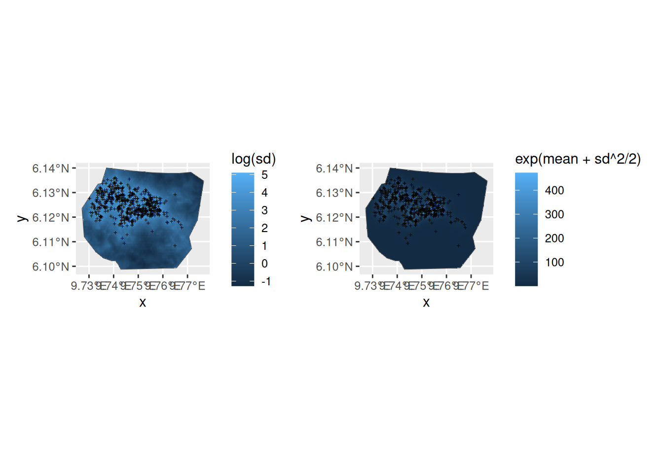

Now look at the elevation and SPDE effects in space. Leave out the Intercept because it swamps the spatial effects of elevation and the SPDE in the plots and we are interested in comparing the effects of elevation and the SPDE.

First we need to predict on the linear predictor scale.

lp_elev_field <- predict(
  fit_elev_field,
  pred.df,
  ~ list(
    smooth_elev = field + elev,
    elev = elev,
    smooth = field
  )
)

The code below, which is very similar to that used for the vegetation factor variable, produces the plots we want.

lprange <- range(
  lp_elev_field$smooth_elev$mean,
  lp_elev_field$elev$mean,
  lp_elev_field$smooth$mean
)

library(RColorBrewer)
csc <- scale_fill_gradientn(colours = brewer.pal(9, "YlOrRd"), limits = lprange)

plot.lp_elev_field <- ggplot() +
  gg(lp_elev_field$smooth_elev, mask = boundary, geom = "tile") +
  csc +
  theme(legend.position = "bottom") +
  gg(boundary, alpha = 0) +
  ggtitle("SPDE + elevation")

plot.lp_elev_field.spde <- ggplot() +
  gg(lp_elev_field$smooth, mask = boundary, geom = "tile") +
  csc +
  gg(boundary, alpha = 0) +
  ggtitle("SPDE")

plot.lp_elev_field.elev <- ggplot() +
  gg(lp_elev_field$elev, mask = boundary, geom = "tile") +
  csc +
  gg(boundary, alpha = 0) +
  ggtitle("elevation")

(plot.lp_elev_field + plot.lp_elev_field.spde + plot.lp_elev_field.elev) +
  plot_layout(ncol = 3, guides = "collect") &
  guides(fill = guide_legend("value")) &
  theme(legend.position = "right")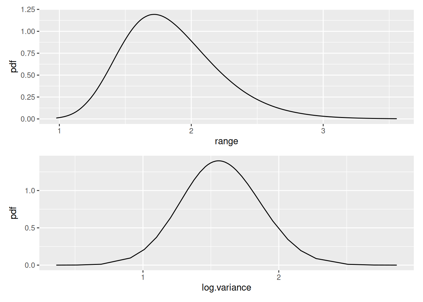

You might also want to look at the posteriors of the fixed effects and of the SPDE. Adapt the code used for the vegetation factor to do this.

Lambda_elev_field <- predict(
  fit_elev_field,
  fm_int(mesh_int, boundary),
  ~ sum(weight * exp(Intercept + elev + field))
)
Lambda_elev_field
#>       mean       sd   q0.025     q0.5   q0.975   median mean.mc_std_err
#> 1 695.9381 30.80826 639.3907 695.0215 756.5462 695.0215        3.566124
#>   sd.mc_std_err
#> 1      2.426492

flist <- vector("list", NROW(fit_elev_field$summary.fixed))
for (i in seq_along(flist)) {
  flist[[i]] <- plot(fit_elev_field, rownames(fit_elev_field$summary.fixed)[i])
  flist_combined <- if (i == 1) flist[[i]] else flist_combined + flist[[i]]
}
flist_combined +
  plot_layout(ncol = 2, guides = "collect")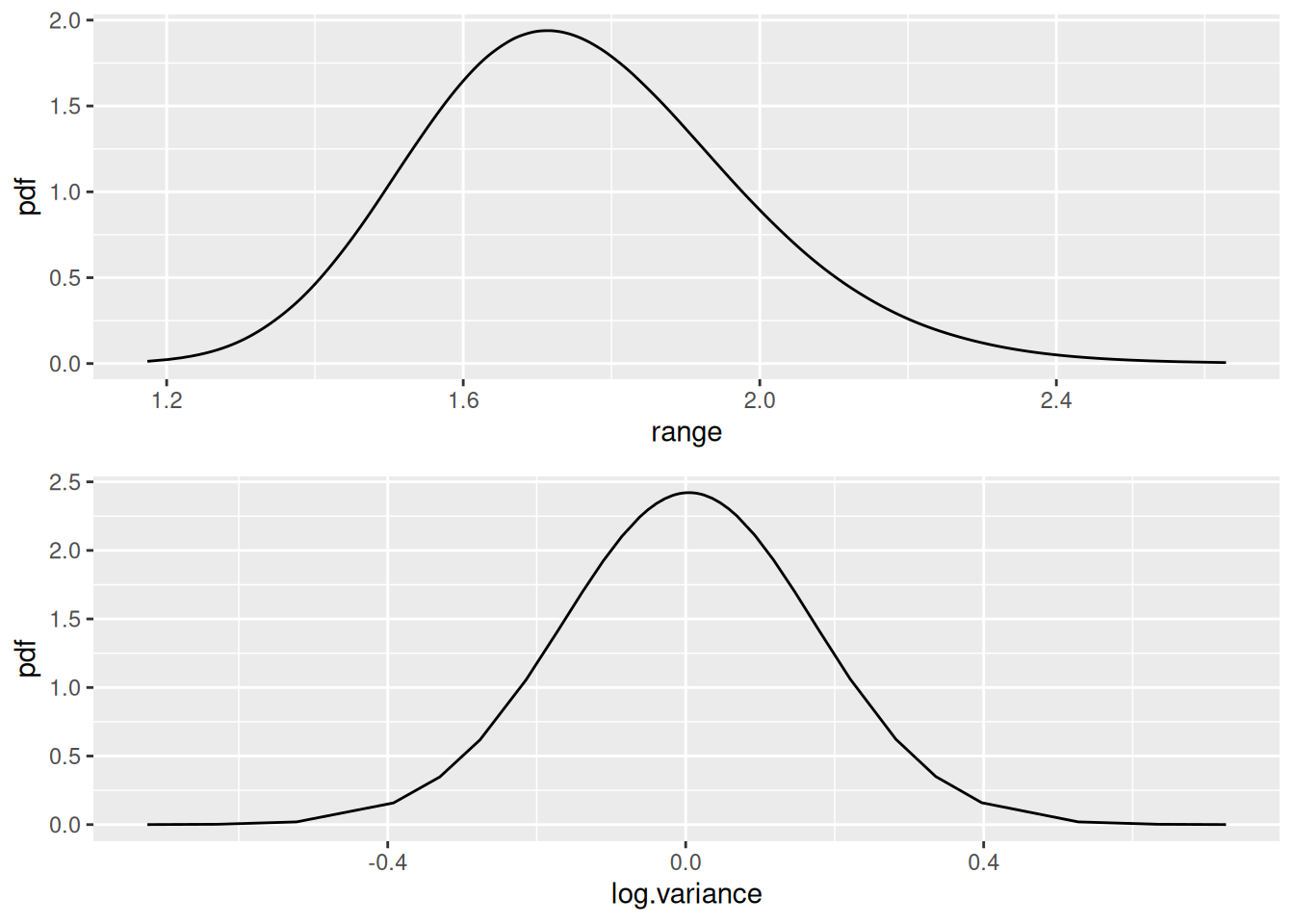

Plot the SPDE parameter posteriors and the Matern correlation and covariance functions for this model.

spde.range <- spde.posterior(fit_elev_field, "field", what = "range")
spde.logvar <- spde.posterior(fit_elev_field, "field", what = "log.variance")
range.plot <- plot(spde.range)
var.plot <- plot(spde.logvar)
(range.plot / var.plot)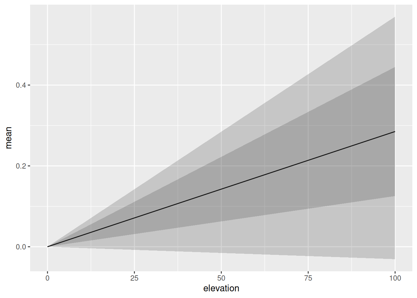


corplot <-
  plot(spde.posterior(fit_elev_field, "field", what = "matern.correlation"))
covplot <-
  plot(spde.posterior(fit_elev_field, "field", what = "matern.covariance"))
(covplot / corplot)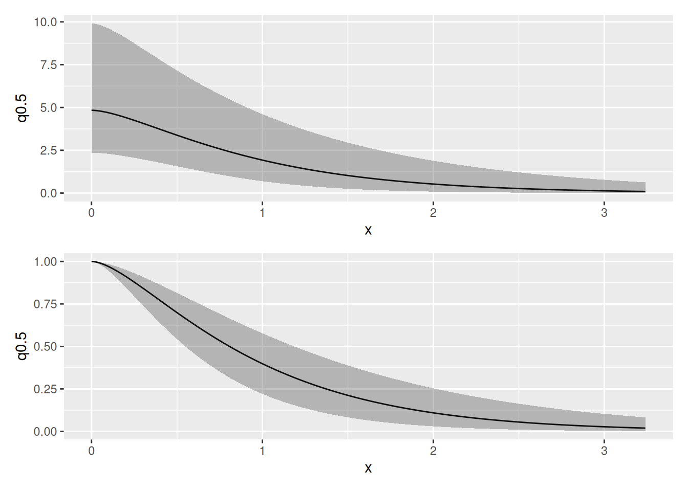

Also estimate abundance. The data.frame in the second call leads to inclusion of N in the prediction object, for easier plotting.

Lambda_elev_field <- predict(
  fit_elev_field, fm_int(mesh_int, boundary),
  ~ sum(weight * exp(field + elev + Intercept))
)
Lambda_elev_field
#>       mean       sd   q0.025     q0.5  q0.975   median mean.mc_std_err
#> 1 694.2443 26.67623 644.6604 693.8146 745.844 693.8146        3.021577
#>   sd.mc_std_err
#> 1      1.769773

Nest_elev_field <- predict(
  fit_elev_field,
  fm_int(mesh_int, boundary),
  ~ data.frame(
    N = 200:1000,
    density = dpois(200:1000,
      lambda = sum(weight * exp(field + elev + Intercept))
    )
  ),
  n.samples = 2000
)

Plot in the same way as in previous practicals

Nest_elev_field$plugin_estimate <-
  dpois(Nest_elev_field$N, lambda = Lambda_elev_field$median)
ggplot(data = Nest_elev_field) +
  geom_line(aes(x = N, y = mean, colour = "Posterior")) +
  geom_line(aes(x = N, y = plugin_estimate, colour = "Plugin"))

Non-spatial evaluation of the covariate effect

The previous examples of posterior prediction focused on spatial prediction. It is also possible to evaluate the effect of a covariate directly, by bypassing the component definition input. This is done by adding the suffix _eval() to the end of the component name in the predictor expression, and supplying data that is sufficient for evaluating , and supplying data needed by the input arguments to this function, see bru_comp_eval().

Note on backwards version support, starting with version 2.2.8 Prior to version 2.8.0, this feature required setting the include argument to character(0) to disable normal component evaluation for all components. From version 2.8.0, inlabru automatically detects which model components are used by the prediction expression, including the use of component _eval() calls, making the include argument unnecessary. From version 2.11.0, the include, exclude, and include_latent arguments have been deprecated in favour of the used argument that takes input generated by bru_used(), with a deprecation warning being generated from version 2.12.0.9003.

Since the elevation effect in this model is linear, the resulting plot isn’t very interesting, but the same method can be applied to non-linear effects (e.g. “rw2”) as well, and combined into general R expressions.

elev.pred <- predict(
  fit_elev_field,
  data.frame(elevation = seq(0, 100, length.out = 1000)),
  formula = ~ elev_eval(elevation)
  # include = character(0) # Not needed from version 2.8.0
)

ggplot(elev.pred) +
  geom_line(aes(elevation, mean)) +
  geom_ribbon(
    aes(elevation,
      ymin = q0.025,
      ymax = q0.975
    ),
    alpha = 0.2
  ) +
  geom_ribbon(
    aes(elevation,
      ymin = mean - 1 * sd,
      ymax = mean + 1 * sd
    ),
    alpha = 0.2
  )

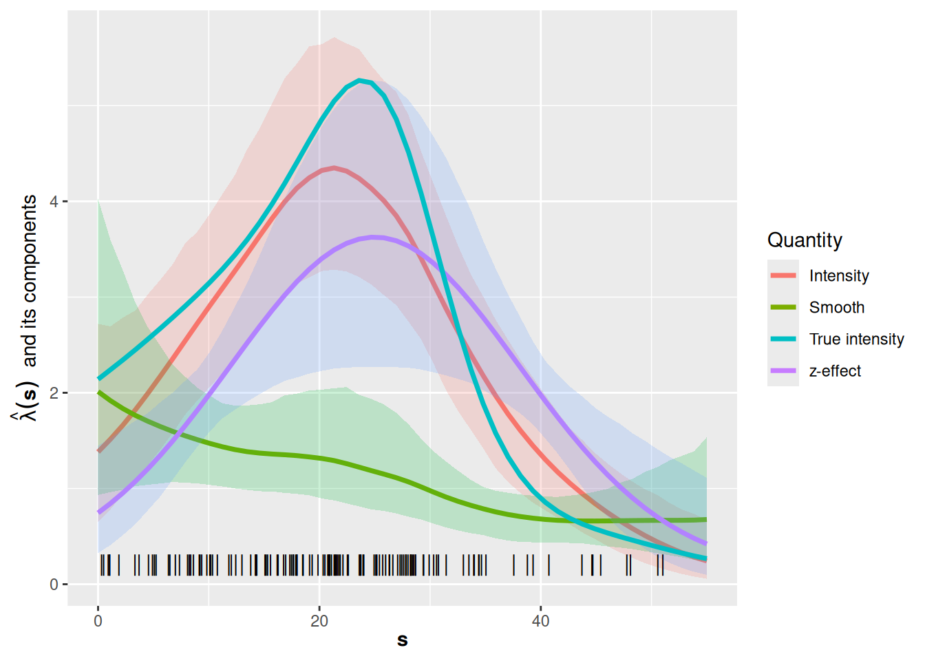
A 1D Example

Try fitting a 1-dimensional model to the point data in the inlabru dataset Poisson2_1D. This comes with a covariate function called cov2_1D. Try to reproduce the plot below (used in lectures) showing the effects of the Intercept + z and the SPDE. (You may find it helpful to build on the model you fitted in the previous practical, adding the covariate to the model specification.)

data(Poisson2_1D)
x <- seq(0, 55, length.out = 50)
mesh <- fm_mesh_1d(x, degree = 2, boundary = "free")

process_model <- inla.spde2.pcmatern(
  mesh,
  prior.sigma = c(1, 0.01),
  prior.range = c(5, 0.01),
  constr = TRUE
)
comp <- x ~
  z(cov2_1D(x), model = "linear") +
  smooth(x, model = process_model) +
  Intercept(1)

fitcov1D <- lgcp(comp,
  pts2,
  domain = list(x = mesh),
  samplers = tibble::tibble(x = cbind(0, 55))
)
pr.df <- data.frame(x = x)
prcov1D <- predict(
  fitcov1D,
  pr.df,
  ~ list(
    Intensity = exp(z + smooth + Intercept),
    z = exp(z + Intercept),
    smooth = exp(smooth)
  ),
  n.samples = 2000
)

ggplot() +
  gg(prcov1D$Intensity,
    aes(colour = "Intensity", fill = "Intensity"),
    alpha = 0.2,
    lwd = 1.25
  ) +
  gg(prcov1D$smooth,
    aes(colour = "Smooth", fill = "Smooth"),
    alpha = 0.2,
    lwd = 1.25
  ) +
  gg(prcov1D$z,
    aes(colour = "z-effect", fill = "z-effect"),
    alpha = 0.2,
    lwd = 1.25
  ) +
  geom_line(aes(x, lambda2_1D(x), colour = "True intensity"), lwd = 1.25) +
  geom_point(data = pts2, aes(x = x), y = 0.2, shape = "|", cex = 4) +
  xlab(quote(bold(s))) +
  ylab(quote(hat(lambda)(bold(s)) ~ ~"and its components")) +
  guides(colour = guide_legend("Quantity"), fill = "none")

LGCPs - Spatial covariates

David Borchers and Finn Lindgren and Hans Montcho

Generated on 2026-05-13