LGCPs - An example in two dimensions • inlabru

Introduction

For this vignette we are going to be working with a dataset obtained from the R package spatstat. We will set up a two-dimensional LGCP to estimate Gorilla abundance.

Setting things up

Load libraries

library(inlabru)
library(INLA)
library(mgcv)
library(ggplot2)

Get the data

For the next few practicals we are going to be working with a dataset obtained from the R package spatstat, which contains the locations of 647 gorilla nests. We load the dataset like this:

data(gorillas_sf, package = "inlabru")

This dataset is a list containing a number of R objects, including the locations of the nests, the boundary of the survey area and an INLA mesh - see help(gorillas) for details. Extract the the objects we need from the list, into other objects, so that we don’t have to keep typing ‘gorillas_sf$’, and optionally load the covariates from disk:

nests <- gorillas_sf$nests
mesh <- gorillas_sf$mesh
boundary <- gorillas_sf$boundary
gcov <- gorillas_sf_gcov()
#> Loading required namespace: terra

Plot the points (the nests).

ggplot() +
  gg(mesh) +
  geom_sf(data = boundary, alpha = 0.1, fill = "blue") +
  geom_sf(data = nests) +
  ggtitle("Points")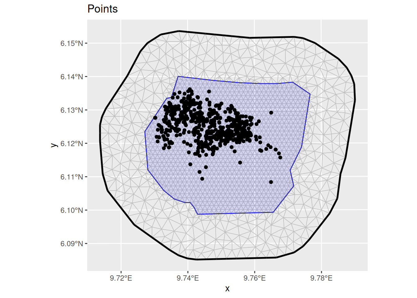

Fitting the model

Fit an LGCP model to the locations of the gorilla nests, predict on the survey region, and produce a plot of the estimated density - which should look like the plot shown below.

The steps to specifying, fitting and predicting are:

Specify a model, comprising (for 2D models) geometry on the left of ~ and an SPDE + Intercept(1) on the right. Please use the SPDE prior specification stated below.
Call lgcp( ), passing it (with 2D models) the model components, the sf containing the observed points and the sf defining the survey boundary using the samplers argument.
Call predict( ), passing it the fitted model from 2., locations at which to predict and an appropriate predictor specification. The locations at which to predict can be a sf covering the mesh, obtained by calling fm_pixels(mesh, format = "sf").

matern <- inla.spde2.pcmatern(
  mesh,
  prior.sigma = c(0.1, 0.01),
  prior.range = c(0.05, 0.01)
)

cmp <- geometry ~
  mySmooth(geometry, model = matern) +
  Intercept(1)

fit <- lgcp(
  cmp,
  data = nests,
  samplers = boundary,
  domain = list(geometry = mesh)
)

Predicting intensity

You should get a plot like that below. The gg method for sf point data takes an optional argument geom = "tile" that converts the plot to the type used for lattice data.

pred <- predict(
  fit,
  fm_pixels(mesh, mask = boundary),
  ~ data.frame(
    lambda = exp(mySmooth + Intercept),
    loglambda = mySmooth + Intercept
  )
)

pl1 <- ggplot() +
  gg(pred$lambda, geom = "tile") +
  geom_sf(data = boundary, alpha = 0.1) +
  ggtitle("LGCP fit to Points", subtitle = "(Response Scale)")

pl2 <- ggplot() +
  gg(pred$loglambda, geom = "tile") +
  geom_sf(data = boundary, alpha = 0.1) +
  ggtitle("LGCP fit to Points", subtitle = "(Linear Predictor Scale)")

multiplot(pl1, pl2, cols = 2)

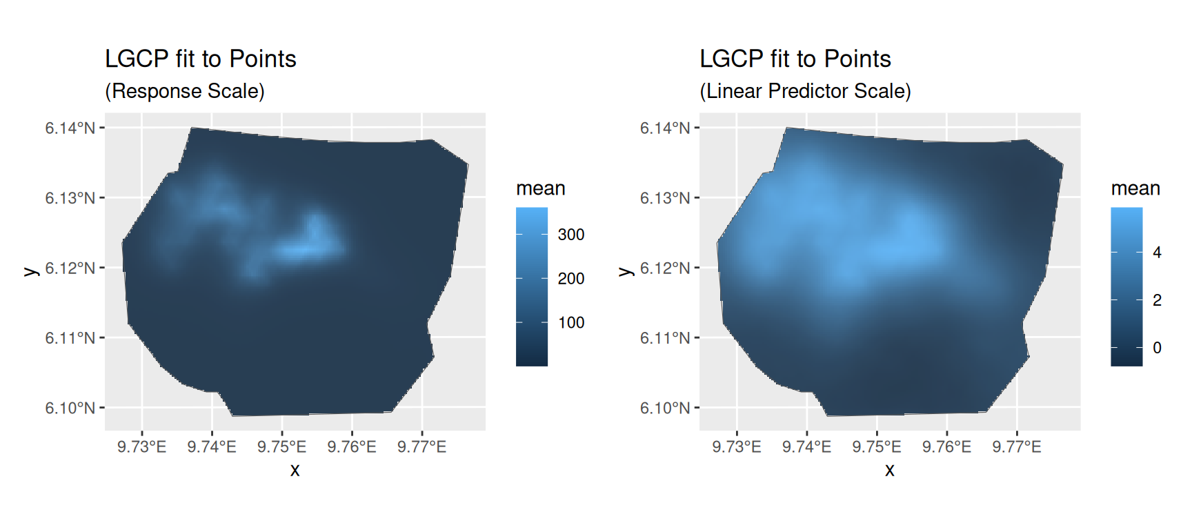
You can plot the median, lower 95% and upper 95% density surfaces as follows (assuming that the predicted intensity is in object lambda).

ggplot() +
  gg(
    tidyr::pivot_longer(pred$lambda,
      c(q0.025, q0.5, q0.975),
      names_to = "quantile", values_to = "value"
    ),
    aes(fill = value),
    geom = "tile"
  ) +
  facet_wrap(~quantile)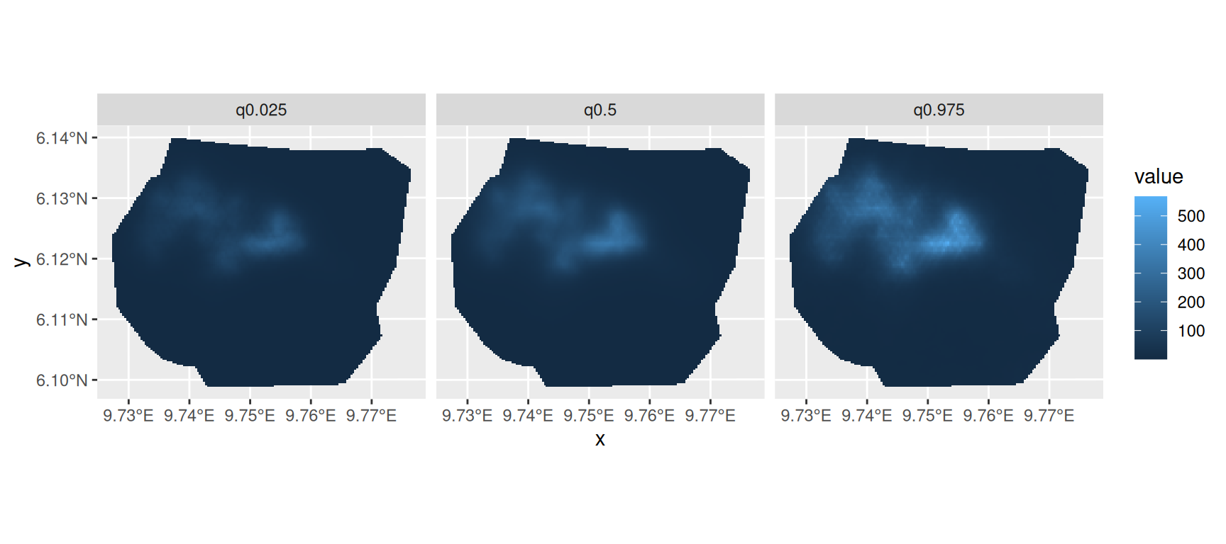

SPDE parameters

Plot the SPDE parameter and fixed effect parameter posteriors.

int.plot <- plot(fit, "Intercept")
spde.range <- spde.posterior(fit, "mySmooth", what = "range")
spde.logvar <- spde.posterior(fit, "mySmooth", what = "log.variance")
range.plot <- plot(spde.range)
var.plot <- plot(spde.logvar)

multiplot(range.plot, var.plot, int.plot)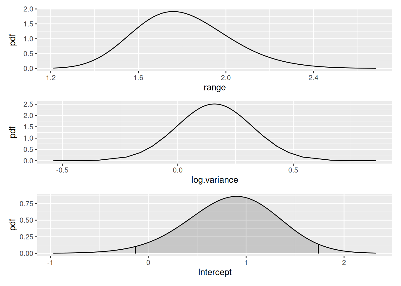

Look at the correlation function if you want to:

corplot <- plot(spde.posterior(fit, "mySmooth", what = "matern.correlation"))
covplot <- plot(spde.posterior(fit, "mySmooth", what = "matern.covariance"))
multiplot(covplot, corplot)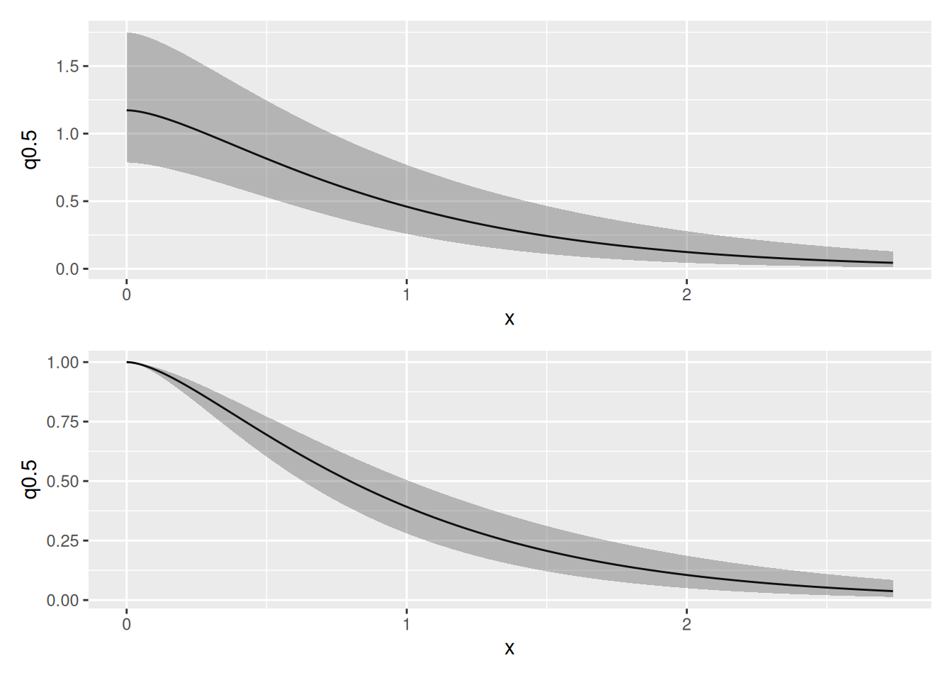

Estimating Abundance

Finally, estimate abundance using the predict function. As a first step we need an estimate for the integrated lambda. The integration weight values are contained in the fm_int() output.

Lambda <- predict(
  fit,
  fm_int(mesh, boundary),
  ~ sum(weight * exp(mySmooth + Intercept))
)
Lambda
#>       mean       sd   q0.025     q0.5   q0.975   median sd.mc_std_err
#> 1 675.2687 23.55334 638.4102 677.2424 720.8927 677.2424      1.943819
#>   mean.mc_std_err
#> 1        2.744098

Given some generous interval boundaries (500, 800) for lambda we can estimate the posterior abundance distribution via

Nest <- predict(
  fit,
  fm_int(mesh, boundary),
  ~ data.frame(
    N = 500:800,
    dpois(500:800,
      lambda = sum(weight * exp(mySmooth + Intercept))
    )
  )
)

Get its quantiles via

inla.qmarginal(c(0.025, 0.5, 0.975), marginal = list(x = Nest$N, y = Nest$mean))
#> [1] 603.6367 672.3612 746.4662

… the mean via

inla.emarginal(identity, marginal = list(x = Nest$N, y = Nest$mean))
#> [1] 673.1795

and plot posteriors:

Nest$plugin_estimate <- dpois(Nest$N, lambda = Lambda$mean)
ggplot(data = Nest) +
  geom_line(aes(x = N, y = mean, colour = "Posterior")) +
  geom_line(aes(x = N, y = plugin_estimate, colour = "Plugin"))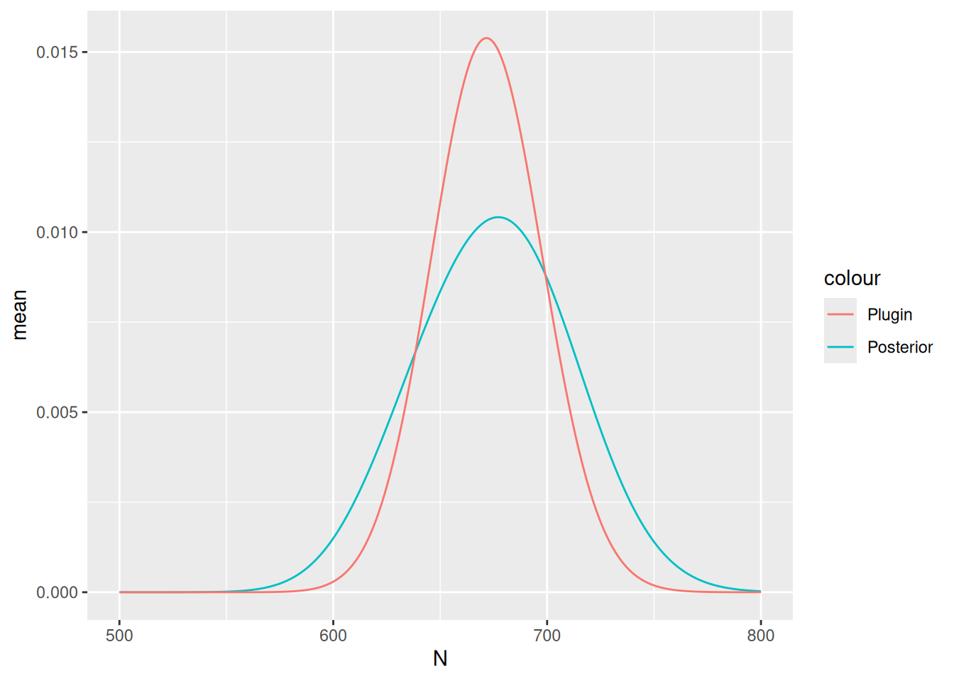

The true number of nests in 647; the mean and median of the posterior distribution of abundance should be close to this if you have not done anything wrong!

LGCPs - An example in two dimensions

David Borchers and Finn Lindgren