Log Gaussian Cox process (LGCP) inference using INLA

This function performs inference on a LGCP observed via points residing possibly multiple dimensions. These dimensions are defined via the left hand side of the formula provided via the model parameter. The left hand side determines the intensity function that is assumed to drive the LGCP. This may include effects that lead to a thinning (filtering) of the point process. By default, the log intensity is assumed to be a linear combination of the effects defined by the formula's RHS.

More sophisticated models, e.g. non-linear thinning, can be achieved by using the predictor argument. The latter requires multiple runs of INLA for improving the required approximation of the predictor. In many applications the LGCP is only observed through subsets of the dimensions the process is living in. For example, spatial point realizations may only be known in sub-areas of the modelled space. These observed subsets of the LGCP domain are called samplers and can be provided via the respective parameter. If samplers is NULL it is assumed that all of the LGCP's dimensions have been observed completely.

Usage

lgcp(
  components,
  data,
  domain = NULL,
  samplers = NULL,
  ips = NULL,
  formula = . ~ .,
  E = NULL,
  weights = NULL,
  ...,
  options = list(),
  .envir = parent.frame()
)

Arguments

components

Latent component definitions, either as a bru_comp_list() object, or a formula-like specification. Also used to define a default linear additive predictor. See bru_comp() for details.

data

Predictor expression-specific data, as a data.frame, tibble, or sf. Since 2.12.0.9023, deprecated support for SpatialPoints[DataFrame] objects.

domain, samplers, ips

Arguments used for family="cp" and aggregate=.

domain

Named list of domain definitions, see fmesher::fm_int().

samplers

Integration domain for family="cp" or subdomains for aggregate=, see fmesher::fm_int().

ips

Integration points. Defaults to fmesher::fm_int(domain, samplers). If explicitly given, overrides domain and samplers.

formula

a formula where the right hand side is a general R expression defines the predictor used in the model.

E

Exposure/effort parameter for family = 'poisson' passed on to INLA::inla. Special case if family is 'cp': rescale all integration weights by a scalar E. For sampler specific reweighting/effort, use a weight column in the samplers object instead, see fmesher::fm_int(). Default taken from options$E, normally 1.

weights

Fixed (optional) weights parameters of the likelihood, so the log-likelihood[i] is changed into weights[i] * log_likelihood[i]. Default value is 1. WARNING: The normalizing constant for the likelihood is NOT recomputed, so ALL marginals (and the marginal likelihood) must be interpreted with great care.

For family = "cp", the weights are applied as sum(weights * eta) in the point location contribution part of the log-likelihood, where eta is the linear predictor, and do not affect the integration part of the likelihood. This can be used to implement approximative methods for point location uncertainty.

...

Further arguments passed on to bru_obs().

options

A bru_options options object or a list of options passed on to bru_options()

.envir

The evaluation environment to use for special arguments (E, Ntrials, weights, and scale) if not found in response_data or data. Defaults to the calling environment.

Value

An bru() object

Details

The E and weights arguments are evaluated in the data context, like for bru_obs().

Examples

# \donttest{
if (bru_safe_inla() &&
  require(ggplot2, quietly = TRUE) &&
  require(fmesher, quietly = TRUE) &&
  require(sn, quietly = TRUE)) {
  # Load the Gorilla data
  data <- gorillas_sf

  # Plot the Gorilla nests, the mesh and the survey boundary
  ggplot() +
    geom_fm(data = data$mesh) +
    gg(data$boundary, fill = "blue", alpha = 0.2) +
    gg(data$nests, col = "red", alpha = 0.2)

  # Define SPDE prior
  matern <- INLA::inla.spde2.pcmatern(
    data$mesh,
    prior.sigma = c(0.1, 0.01),
    prior.range = c(0.1, 0.01)
  )

  # Define domain of the LGCP as well as the model components (spatial SPDE
  # effect and Intercept)
  cmp <- geometry ~ field(geometry, model = matern) + Intercept(1)

  # Fit the model (with int.strategy="eb" to make the example take less time)
  fit <- lgcp(cmp, data$nests,
    samplers = data$boundary,
    domain = list(geometry = data$mesh),
    options = list(control.inla = list(int.strategy = "eb"))
  )

  # Predict the spatial intensity surface
  lambda <- predict(
    fit,
    fm_pixels(data$mesh, mask = data$boundary),
    ~ exp(field + Intercept)
  )

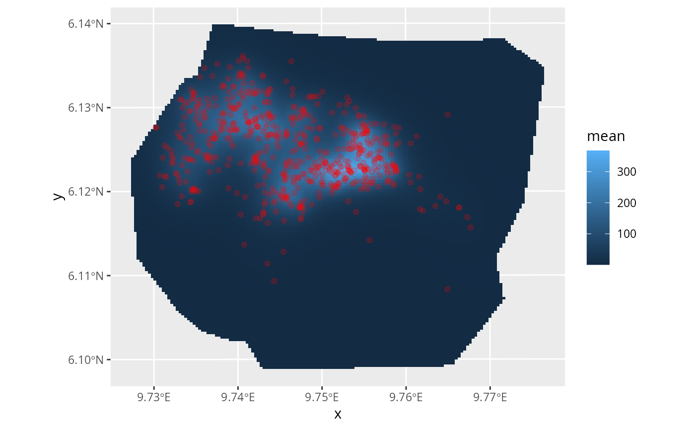
  # Plot the intensity
  ggplot() +
    gg(lambda, geom = "tile") +
    geom_fm(data = data$mesh, alpha = 0, linewidth = 0.05) +
    gg(data$nests, col = "red", alpha = 0.2)
}

# }