LGCPs - An example in space and time

Fabian E. Bachl and Finn Lindgren

Generated on 2025-02-15

Introduction

For this vignette we are going to be working with a dataset obtained from the R package MRSea. We will set up a LGCP with a spatio-temporal SPDE model to estimate species distribution.

Setting things up

Load libraries

library(inlabru)
library(INLA)
library(ggplot2)

Get the data

Load the dataset, that has coordinates in UTM in kilometres:

mrsea <- inlabru::mrsea

The points (representing animals) and the sampling regions of this dataset are associated with a season. Let’s have a look at the observed points and sampling regions for all seasons:

ggplot() +
  geom_fm(data = mrsea$mesh) +
  gg(mrsea$boundary) +
  gg(mrsea$samplers) +
  gg(mrsea$points, size = 0.5) +
  facet_wrap(~season) +
  ggtitle("MRSea observation seasons")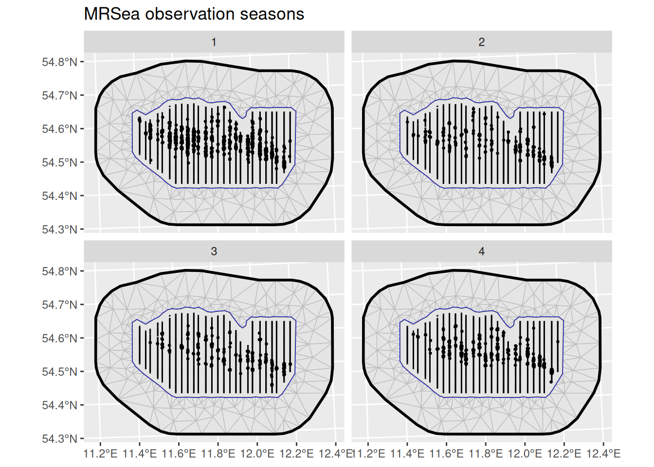

Fitting the model

Fit an LGCP model to the locations of the animals. In this example we will employ a spatio-temporal SPDE. Note how the group and ngroup parameters are employed to let the SPDE model know about the name of the time dimension (season) and the total number of distinct points in time. The point process likelihood is constructed by the lgcp() function, which is a wrapper around the bru_obs(..., model = "cp") and bru() functions. Like for ordinary spatial point process models, the samplers argument specifies the observation region/set, in this case combinations spatial lines and seasons. The domain argument specifies the spatio-temporal function space to use when constructing the numerical integration scheme needed for the point process likelihood evaluation.

matern <- inla.spde2.pcmatern(mrsea$mesh,
  prior.sigma = c(0.1, 0.01),
  prior.range = c(10, 0.01)
)

cmp <- geometry + season ~ Intercept(1) +
  mySmooth(
    geometry,
    model = matern,
    group = season,
    ngroup = 4
  )

fit <- lgcp(cmp,
  data = mrsea$points,
  samplers = mrsea$samplers,
  domain = list(
    geometry = mrsea$mesh,
    season = seq_len(4)
  )
)

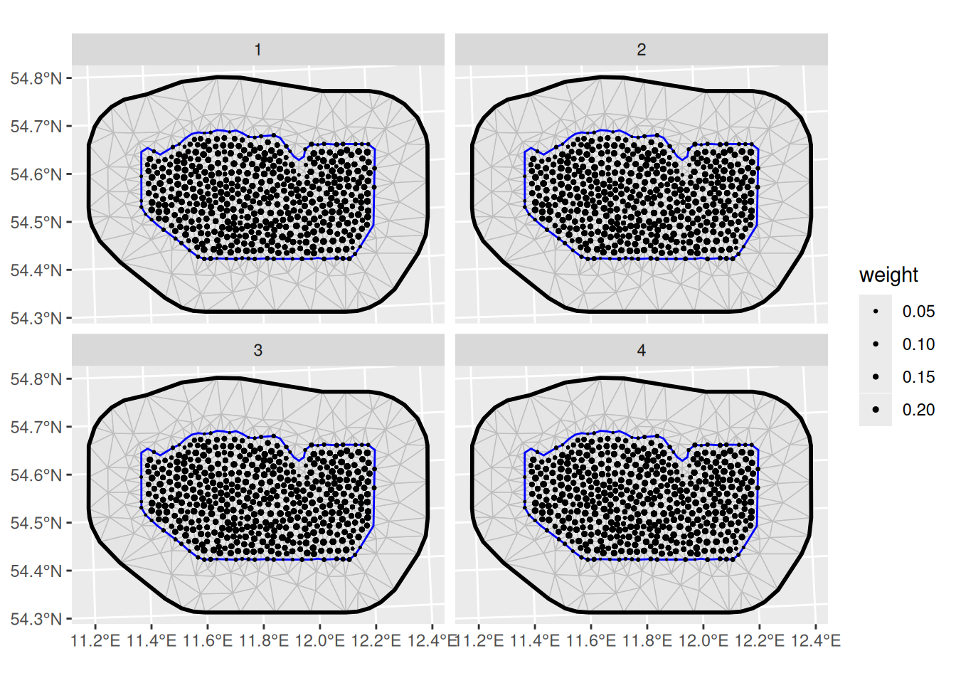
Predict and plot the intensity for all seasons:

ppxl <- fm_pixels(mrsea$mesh, mask = mrsea$boundary, format = "sf")
ppxl_all <- fm_cprod(ppxl, data.frame(season = seq_len(4)))

lambda1 <- predict(
  fit,
  ppxl_all,
  ~ data.frame(season = season, lambda = exp(mySmooth + Intercept))
)

pl1 <- ggplot() +
  gg(lambda1, geom = "tile", aes(fill = q0.5)) +
  gg(mrsea$points, size = 0.3) +
  facet_wrap(~season) +
  coord_sf()
pl1

Integration points

The inlabru point process model, lgcp() or bru_obs(..., model = "cp"), knows how to construct the numerical integration scheme for the LGCP likelihood. To see what happens internally, we can also call the internal functions directly to see what the integration scheme will look like, using the fm_int() function with the same domain and samplers arguments as in the previous lgcp() call. Note that omitting the season dimension from domain would lead to aggregation of all sampling regions over time.

ips <- fm_int(
  domain = list(geometry = mrsea$mesh, season = 1:4),
  samplers = mrsea$samplers
)

Plot the integration points:

ggplot() +
  geom_fm(data = mrsea$mesh) +
  gg(ips, aes(size = weight)) +
  scale_size_area(max_size = 1) +
  facet_wrap(~season)