LGCPs - Distance sampling • inlabru

Introduction

We’re going to estimate distribution and abundance from a line transect survey of dolphins in the Gulf of Mexico. These data are also available in the R package dsm (where they go under the name mexdolphins). In inlabru the data are called mexdolphin for sp format, and mexdolphin_sf for sf format.

Setting things up

Load libraries

library(inlabru)
library(fmesher)
library(INLA)
library(ggplot2)

Get the data

We’ll start by loading the data, renaming it, and extracting the mesh (for convenience).

mexdolphin <- mexdolphin_sf
mesh <- mexdolphin$mesh

Plot the data (the initial code below is just to get rid of tick marks, if desired)

noyticks <- theme(
  axis.text.y = element_blank(),
  axis.ticks = element_blank()
)

noxticks <- theme(
  axis.text.x = element_blank(),
  axis.ticks = element_blank()
)

ggplot() +
  gg(mexdolphin$ppoly) +
  gg(mexdolphin$samplers, color = "grey") +
  gg(mexdolphin$points, size = 0.2, alpha = 1) +
  theme(legend.key.width = unit(x = 0.2, "cm"), legend.key.height = unit(x = 0.3, "cm")) +
  theme(legend.text = element_text(size = 6))

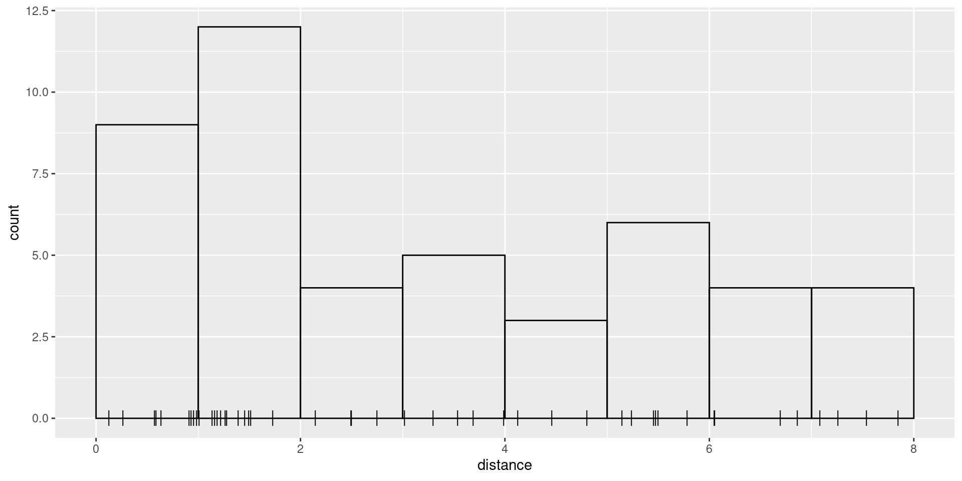
Spatial model with a half-normal detection function

The samplers in this dataset are lines, not polygons, so we need to tell inlabru about the strip half-width, W, which in the case of these data is 8. We start by plotting the distances and histogram of frequencies in distance intervals:

W <- 8
ggplot(mexdolphin$points) +
  geom_histogram(aes(x = distance),
    breaks = seq(0, W, length.out = 9),
    boundary = 0, fill = NA, color = "black"
  ) +
  geom_point(aes(x = distance), y = 0, pch = "|", cex = 4)

We need to define a half-normal detection probability function. This must take distance as its first argument and the linear predictor of the sigma parameter as its second:

hn <- function(distance, sigma) {
  exp(-0.5 * (distance / sigma)^2)
}

To control the prior distribution for the sigma parameter, we define a transformation function that converts a \(N(0, 1)\) latent variable into an exponentially distributed variable with expectation 8 (this is a somewhat arbitrary value, but motivated by the maximum observation distance W):

sigma <- function(x) {
  bru_forward_transformation(qexp, x, rate = 1 / 8)
}

Specify and fit an SPDE model to these data using a half-normal detection function form. We need to define a (Matérn) covariance function for the SPDE

matern <- inla.spde2.pcmatern(mexdolphin$mesh,
  prior.sigma = c(2, 0.01),
  prior.range = c(50, 0.01)
)

We need to now separately define the components of the model (the SPDE, the Intercept and the detection function parameter sigma_theta)

cmp <- ~ mySPDE(main = geometry, model = matern) +
  sigma_theta(1, prec.linear = 1) + Intercept(1)

… and the formula, which describes how these components are combined to form the linear predictor (remembering that we need an offset due to the unknown direction of the detections!):

form <- geometry + distance ~ mySPDE +
  log(hn(distance, sigma(sigma_theta))) +
  Intercept + log(2)

From version 2.9.0.9004, a more compact option is available, by allowing the component itself do the transformation between N(0,1) and Exponential(1/8):

# # An alternative approach available from 2.9.0.9004; requires matching
# # adjustments to the later predict() calls, etc.
# cmp <- ~ mySPDE(main = geometry, model = matern) +
#   sigma(1,
#     prec.linear = 1,
#     marginal = bru_mapper_marginal(qexp, pexp, dexp, rate = 1 / 8)
#   ) +
#   Intercept(1)
# form <- geometry + distance ~ mySPDE +
#   log(hn(distance, sigma)) +
#   Intercept + log(2)

Then we fit the model, passing both the components and the formula (previously the formula was constructed invisibly by inlabru), and specify integration domains for the spatial and distance dimensions:

fit <- lgcp(
  components = cmp,
  mexdolphin$points,
  samplers = mexdolphin$samplers,
  domain = list(
    geometry = mesh,
    distance = fm_mesh_1d(seq(0, 8, length.out = 30))
  ),
  formula = form
)

Look at the SPDE parameter posteriors

spde.range <- spde.posterior(fit, "mySPDE", what = "range")
plot(spde.range)

spde.logvar <- spde.posterior(fit, "mySPDE", what = "log.variance")
plot(spde.logvar)

Predict spatial intensity, and plot it:

pxl <- fm_pixels(mesh, dims = c(200, 100), mask = mexdolphin$ppoly)
pr.int <- predict(fit, pxl, ~ exp(mySPDE + Intercept))

ggplot() +
  gg(pr.int, geom = "tile") +
  gg(mexdolphin$ppoly, linewidth = 1, alpha = 0) +
  gg(mexdolphin$samplers, color = "grey") +
  gg(mexdolphin$points, size = 0.2, alpha = 1) +
  theme(legend.key.width = unit(x = 0.2, "cm"), legend.key.height = unit(x = 0.3, "cm")) +
  theme(legend.text = element_text(size = 6))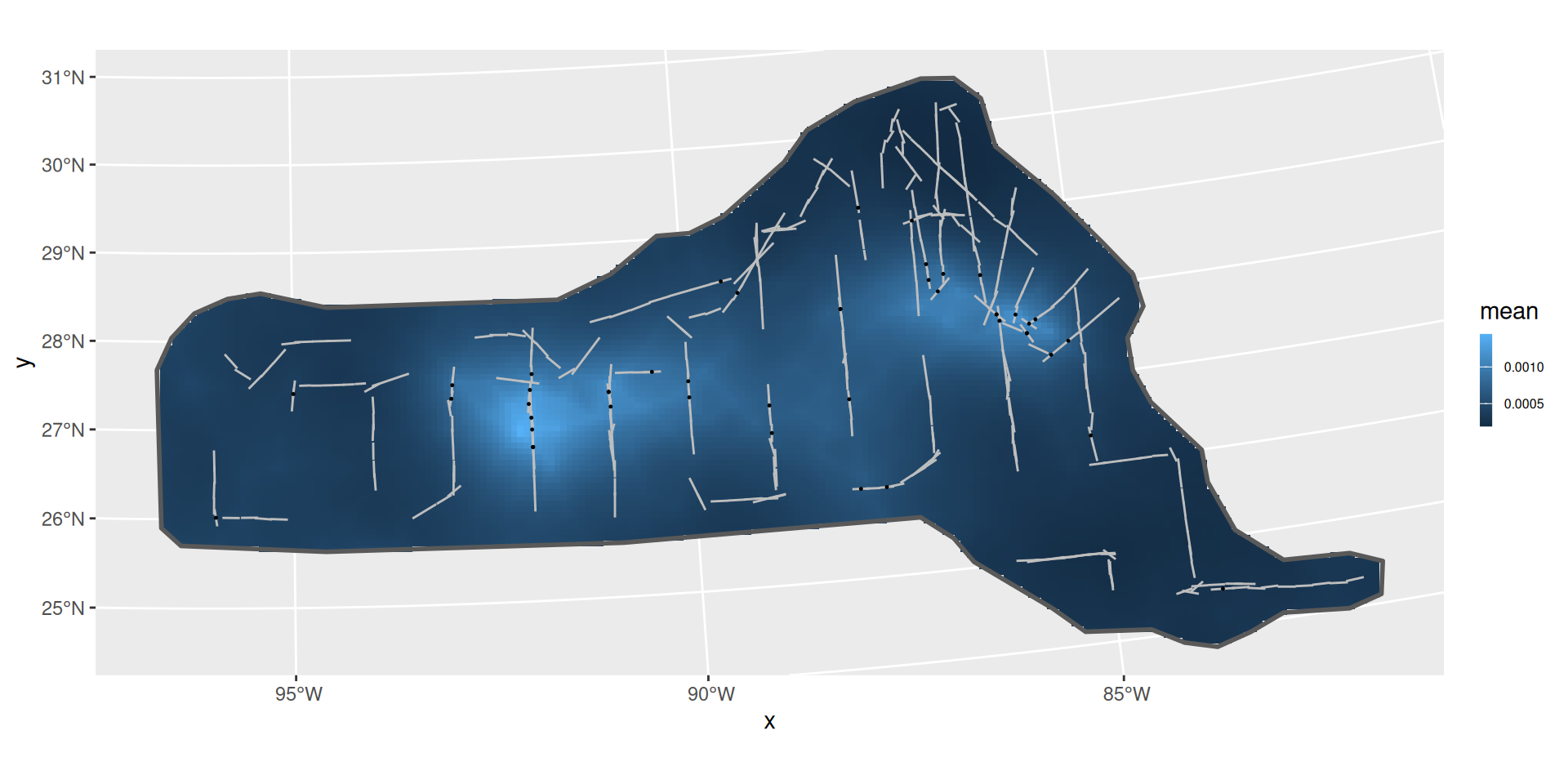

Predict the detection function and plot it, to generate a plot like the one below. Here, we should make sure that it doesn’t try to evaluate the effects of components that can’t be evaluated using the given input data. From version 2.8.0, inlabru automatically detects which components are involved. See ?predict.bru for more information.

distdf <- data.frame(distance = seq(0, 8, length.out = 100))
dfun <- predict(fit, distdf, ~ hn(distance, sigma(sigma_theta)))
plot(dfun)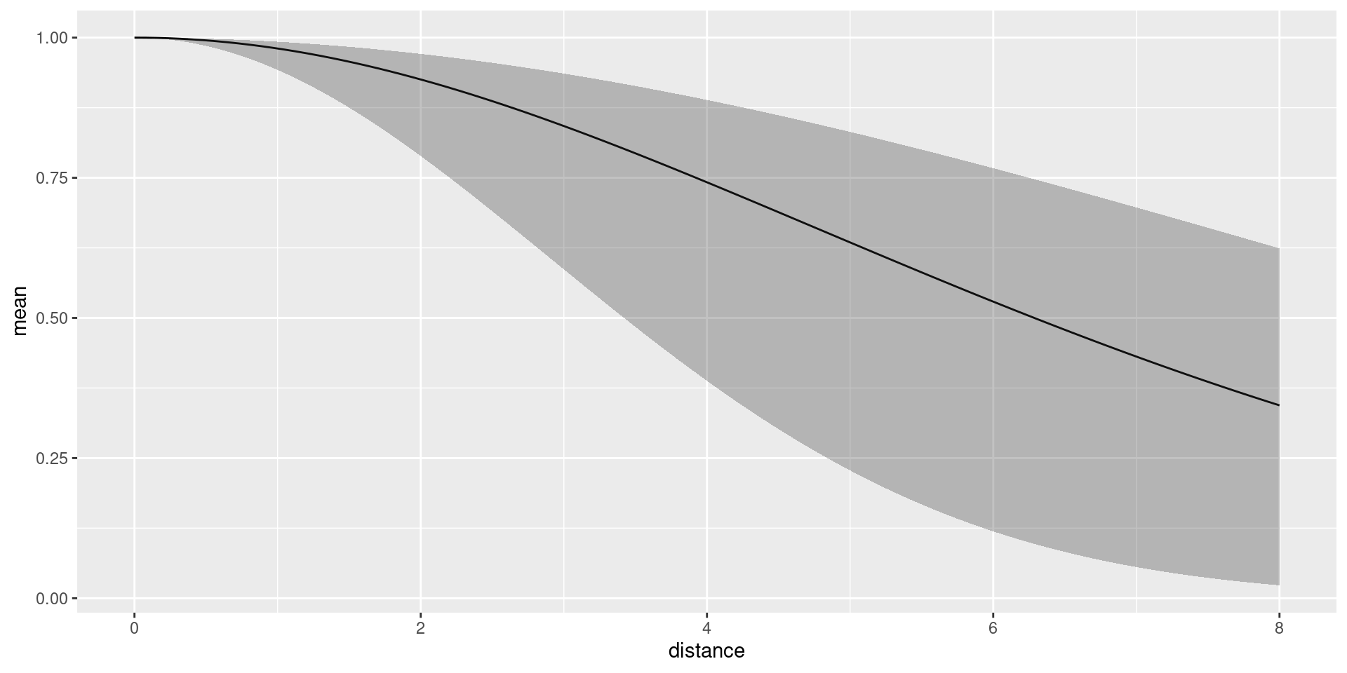

The average detection probability within the maximum detection distance is estimated to be 0.7051994.

We can look at the posterior for expected number of dolphins as usual:

predpts <- fm_int(mexdolphin$mesh, mexdolphin$ppoly)
Lambda <- predict(fit, predpts, ~ sum(weight * exp(mySPDE + Intercept)))
Lambda
#>       mean       sd   q0.025     q0.5   q0.975   median mean.mc_std_err
#> 1 235.0928 48.00858 150.3372 237.8767 328.8852 237.8767        4.800858
#>   sd.mc_std_err
#> 1      2.925312

and including the randomness about the expected number. In this case, it turns out that you need lots of posterior samples, e.g. 2,000 to smooth out the Monte Carlo error in the posterior, and this takes a little while to compute:

Ns <- seq(50, 450, by = 1)
Nest <- predict(fit, predpts,
  ~ data.frame(
    N = Ns,
    density = dpois(Ns,
      lambda = sum(weight * exp(mySPDE + Intercept))
    )
  ),
  n.samples = 2000
)

Nest$plugin_estimate <- dpois(Nest$N, lambda = Lambda$mean)
ggplot(data = Nest) +
  geom_line(aes(x = N, y = mean, colour = "Posterior")) +
  geom_ribbon(
    aes(
      x = N,
      ymin = mean - 2 * mean.mc_std_err,
      ymax = mean + 2 * mean.mc_std_err,
      colour = NULL, fill = "Posterior"
    ),
    alpha = 0.2
  ) +
  geom_line(aes(x = N, y = plugin_estimate, colour = "Plugin", fill = "Plugin"))

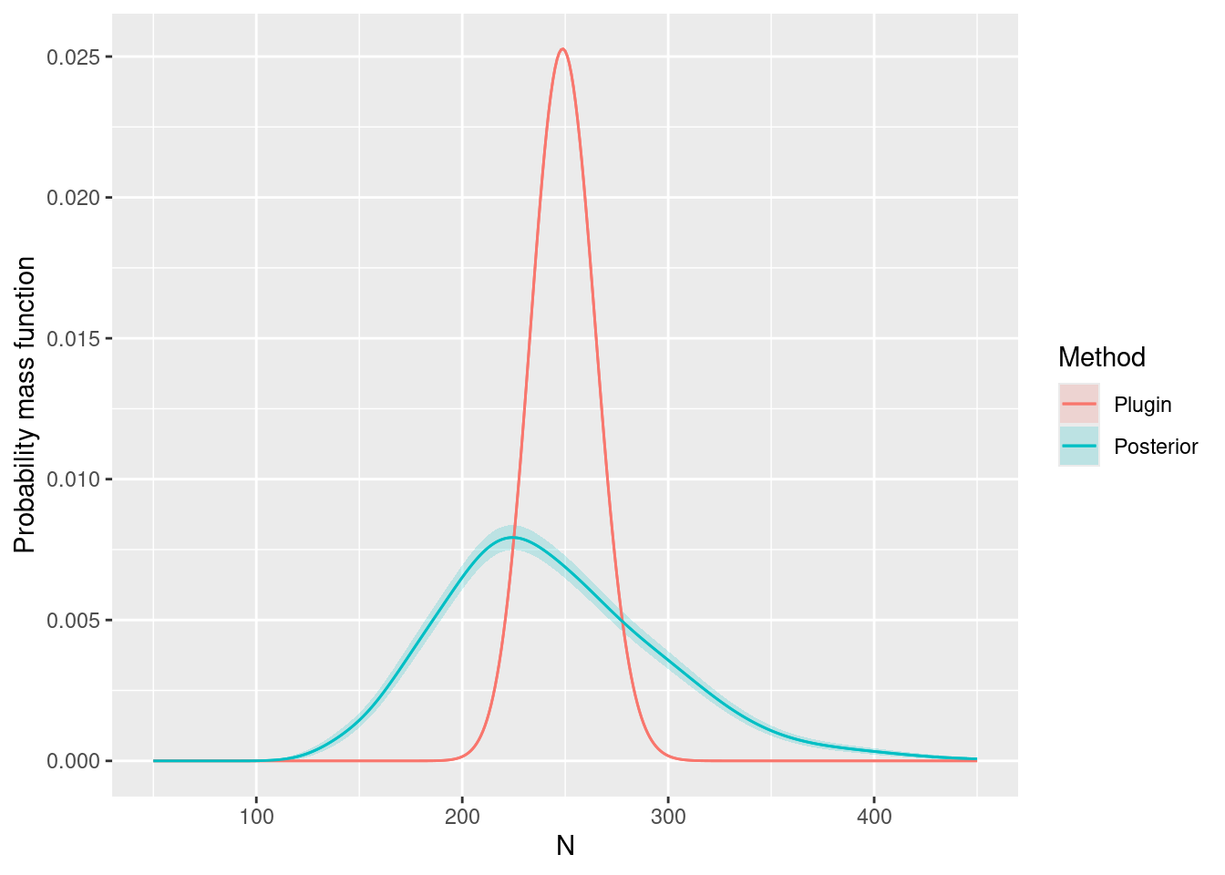
Hazard-rate Detection Function

Try doing this all again, but use this hazard-rate detection function model, with the same prior for the sigma parameter as for the half-Normal model (such parameters aren’t always comparable, but in this example it’s a reasonable choice):

hr <- function(distance, sigma) {
  1 - exp(-(distance / sigma)^-1)
}

Solution:

formula1 <- geometry + distance ~ mySPDE +
  log(hr(distance, sigma(sigma_theta))) +
  Intercept + log(2)

fit1 <- lgcp(
  components = cmp,
  mexdolphin$points,
  samplers = mexdolphin$samplers,
  domain = list(
    geometry = mesh,
    distance = fm_mesh_1d(seq(0, 8, length.out = 30))
  ),
  formula = formula1
)

Plots:

spde.range <- spde.posterior(fit1, "mySPDE", what = "range")
plot(spde.range)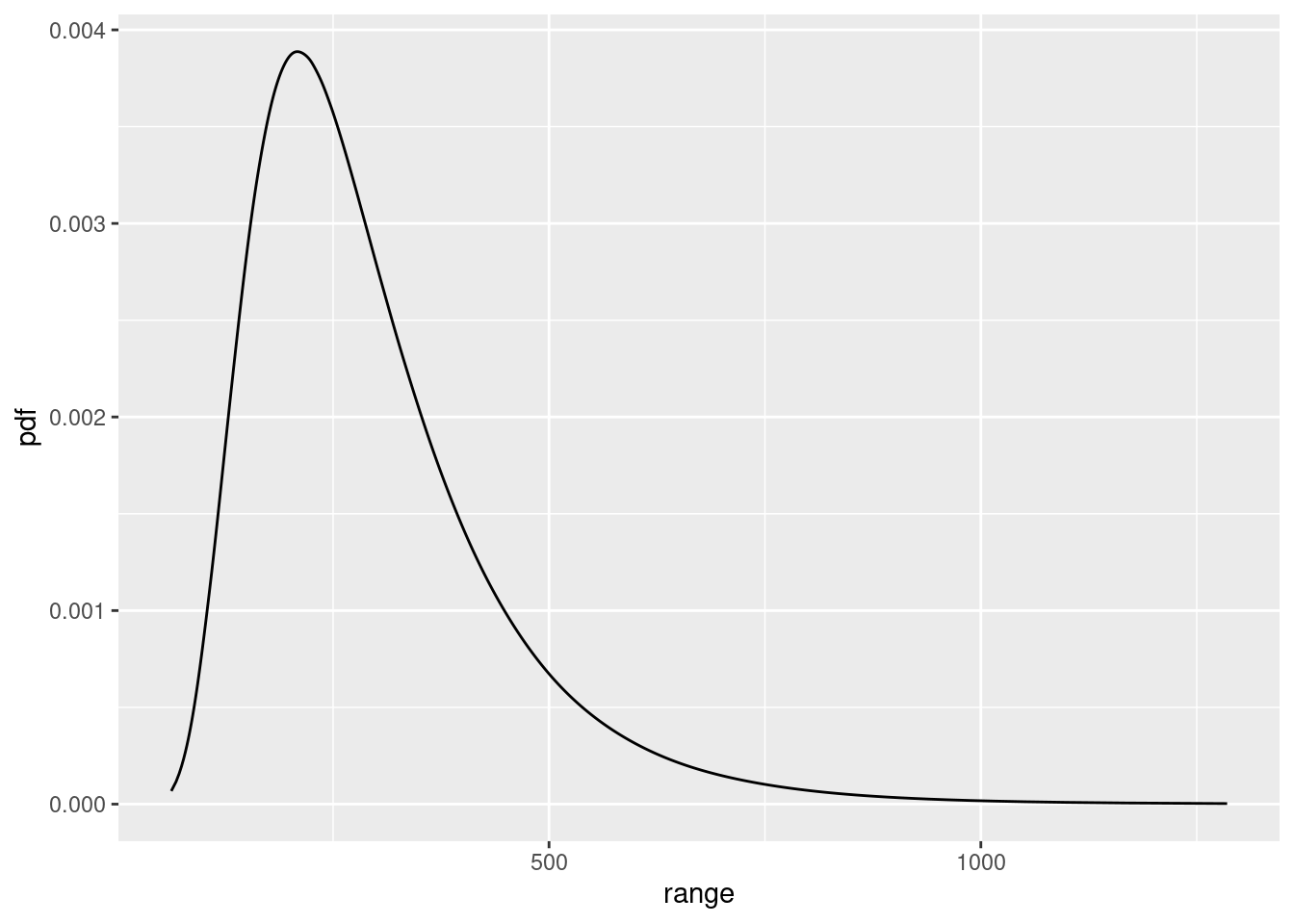

spde.logvar <- spde.posterior(fit1, "mySPDE", what = "log.variance")
plot(spde.logvar)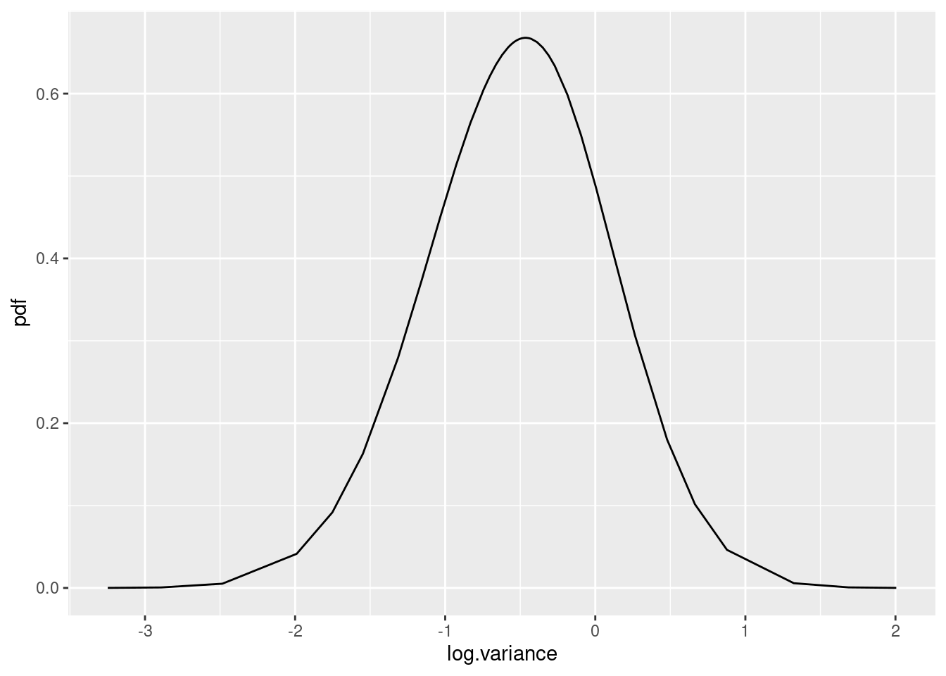


pr.int1 <- predict(fit1, pxl, ~ exp(mySPDE + Intercept))

ggplot() +
  gg(pr.int1, geom = "tile") +
  gg(mexdolphin$ppoly, linewidth = 1, alpha = 0) +
  gg(mexdolphin$samplers, color = "grey") +
  gg(mexdolphin$points, size = 0.2, alpha = 1) +
  theme(legend.key.width = unit(x = 0.2, "cm"), legend.key.height = unit(x = 0.3, "cm")) +
  theme(legend.text = element_text(size = 6))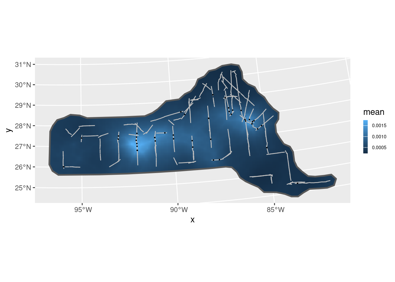


distdf <- data.frame(distance = seq(0, 8, length.out = 100))
dfun1 <- predict(fit1, distdf, ~ hr(distance, sigma(sigma_theta)))
plot(dfun1)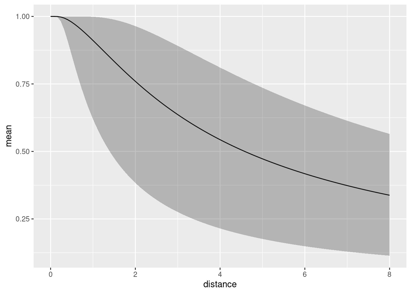


predpts <- fm_int(mexdolphin$mesh, mexdolphin$ppoly)
Lambda1 <- predict(fit1, predpts, ~ sum(weight * exp(mySPDE + Intercept)))
Lambda1
#>       mean       sd   q0.025     q0.5  q0.975   median mean.mc_std_err
#> 1 294.7596 99.25167 152.3689 267.4158 481.443 267.4158        9.925167
#>   sd.mc_std_err
#> 1      7.107299

Ns <- seq(50, 650, by = 1)
Nest1 <- predict(
  fit1,
  predpts,
  ~ data.frame(
    N = Ns,
    density = dpois(Ns,
      lambda = sum(weight * exp(mySPDE + Intercept))
    )
  ),
  n.samples = 2000
)

Nest1$plugin_estimate <- dpois(Nest1$N, lambda = Lambda1$mean)
ggplot(data = Nest1) +
  geom_line(aes(x = N, y = mean, colour = "Posterior")) +
  geom_ribbon(
    aes(
      x = N,
      ymin = mean - 2 * mean.mc_std_err,
      ymax = mean + 2 * mean.mc_std_err,
      colour = NULL, fill = "Posterior"
    ),
    alpha = 0.2
  ) +
  geom_line(aes(x = N, y = plugin_estimate, colour = "Plugin", fill = "Plugin"))

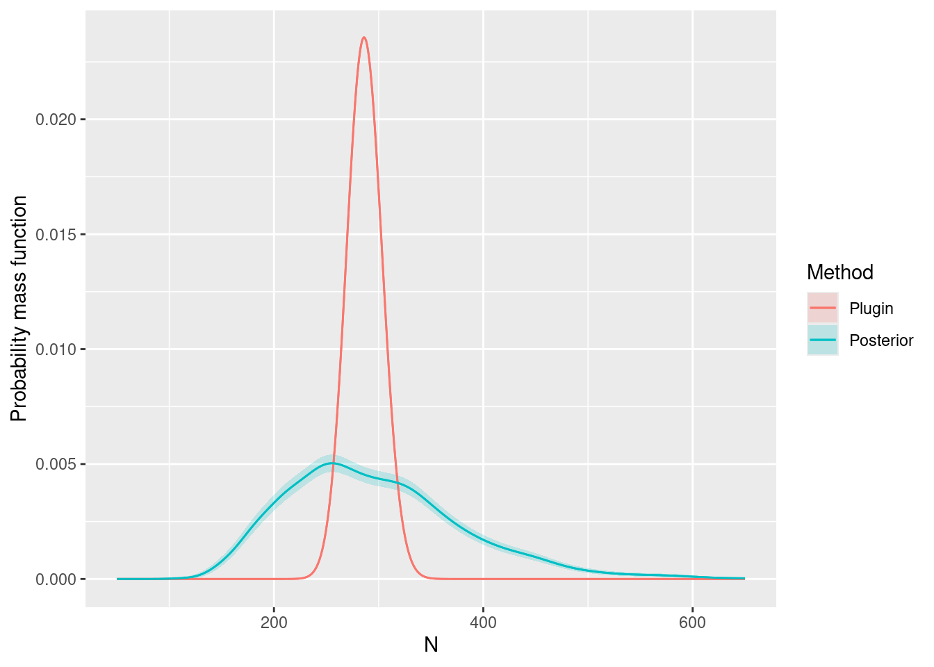
Comparing the models

Look at the goodness-of-fit of the two models in the distance dimension

bc <- bincount(
  result = fit,
  observations = mexdolphin$points$distance,
  breaks = seq(0, max(mexdolphin$points$distance), length.out = 9),
  predictor = distance ~ hn(distance, sigma(sigma_theta))
)
attributes(bc)$ggp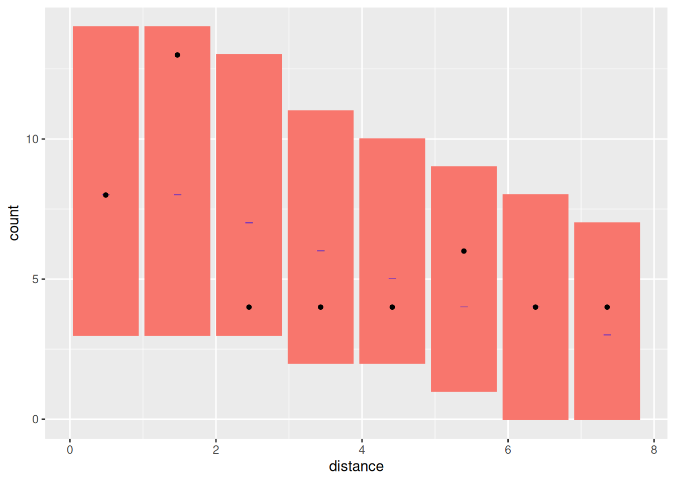


bc1 <- bincount(
  result = fit1,
  observations = mexdolphin$points$distance,
  breaks = seq(0, max(mexdolphin$points$distance), length.out = 9),
  predictor = distance ~ hn(distance, sigma(sigma_theta))
)
attributes(bc1)$ggp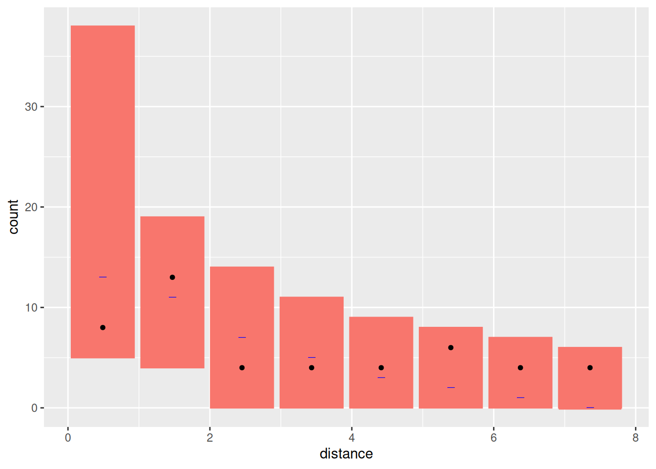

Fit Models only to the distance sampling data

Half-normal first

formula <- distance ~ log(hn(distance, sigma(sigma_theta))) + Intercept
cmp <- ~ sigma_theta(1, prec.linear = 1) + Intercept(1)
dfit <- lgcp(
  components = cmp,
  mexdolphin$points,
  domain = list(distance = fm_mesh_1d(seq(0, 8, length.out = 30))),
  formula = formula,
  options = list(bru_initial = list(sigma_theta = 1, Intercept = 3))
)
detfun <- predict(dfit, distdf, ~ hn(distance, sigma(sigma_theta)))

Hazard-rate next

formula1 <- distance ~ log(hr(distance, sigma(sigma_theta))) + Intercept
cmp <- ~ sigma_theta(1, prec.linear = 1) + Intercept(1)
dfit1 <- lgcp(
  components = cmp,
  mexdolphin$points,
  domain = list(distance = fm_mesh_1d(seq(0, 8, length.out = 30))),
  formula = formula1
)
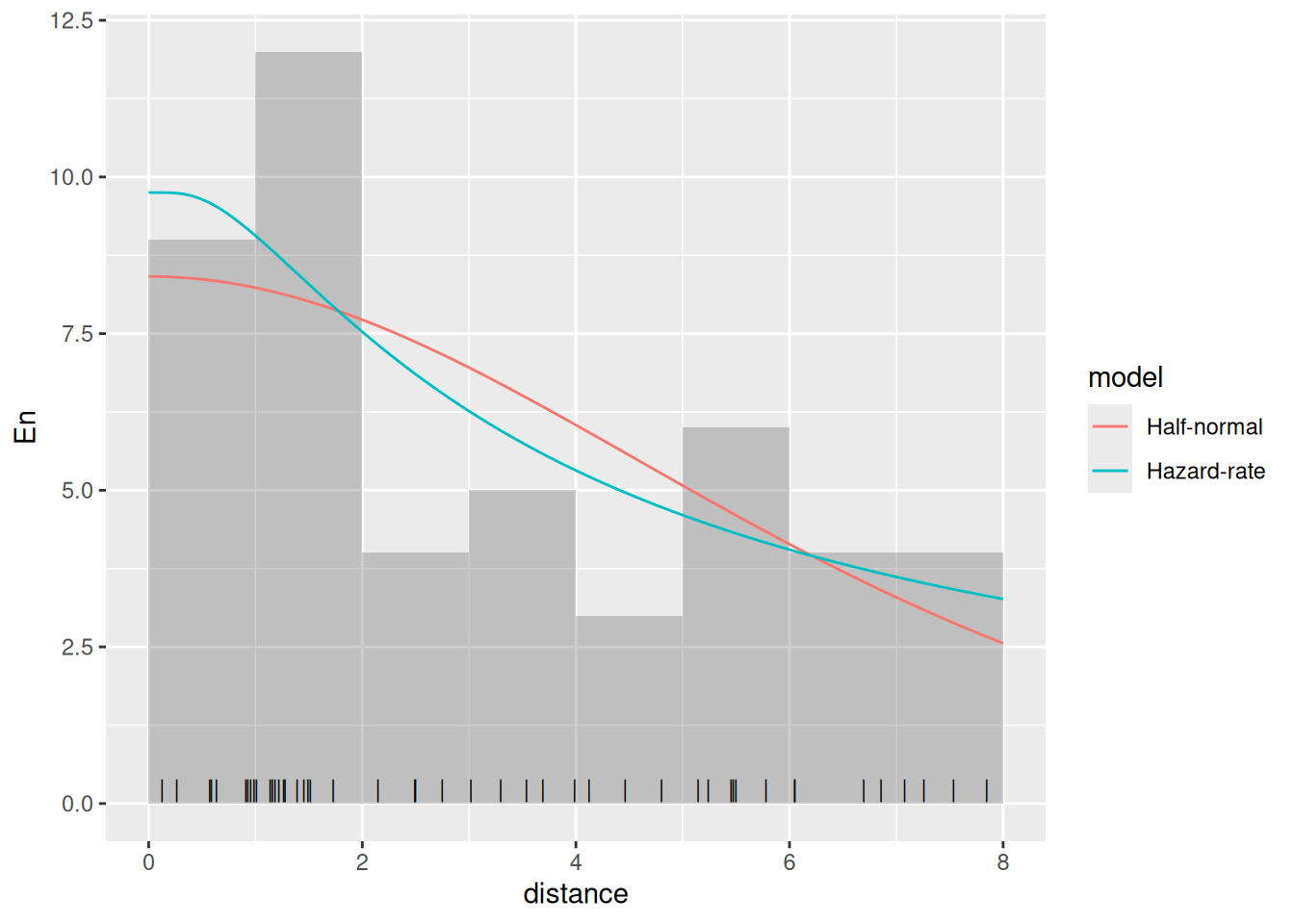
detfun1 <- predict(dfit1, distdf, ~ hr(distance, sigma(sigma_theta)))

Plot both lines on histogram of observations. First scale lines to have same area as that of histogram.

Half-normal:

hnline <- data.frame(distance = detfun$distance, p = detfun$mean, lower = detfun$q0.025, upper = detfun$q0.975)
wts <- diff(hnline$distance)
wts[1] <- wts[1] / 2
wts <- c(wts, wts[1])
hnarea <- sum(wts * hnline$p)
n <- length(mexdolphin$points$distance)
scale <- n / hnarea
hnline$En <- hnline$p * scale
hnline$En.lower <- hnline$lower * scale
hnline$En.upper <- hnline$upper * scale

Hazard-rate:

hrline <- data.frame(distance = detfun1$distance, p = detfun1$mean, lower = detfun1$q0.025, upper = detfun1$q0.975)
wts <- diff(hrline$distance)
wts[1] <- wts[1] / 2
wts <- c(wts, wts[1])
hrarea <- sum(wts * hrline$p)
n <- length(mexdolphin$points$distance)
scale <- n / hrarea
hrline$En <- hrline$p * scale
hrline$En.lower <- hrline$lower * scale
hrline$En.upper <- hrline$upper * scale

Combine lines in a single object for plotting

dlines <- rbind(
  cbind(hnline, model = "Half-normal"),
  cbind(hrline, model = "Hazard-rate")
)

Plot without the 95% credible intervals

ggplot(data.frame(mexdolphin$points)) +
  geom_histogram(aes(x = distance), breaks = seq(0, 8, length.out = 9), alpha = 0.3) +
  geom_point(aes(x = distance), y = 0.2, shape = "|", size = 3) +
  geom_line(data = dlines, aes(x = distance, y = En, group = model, col = model))

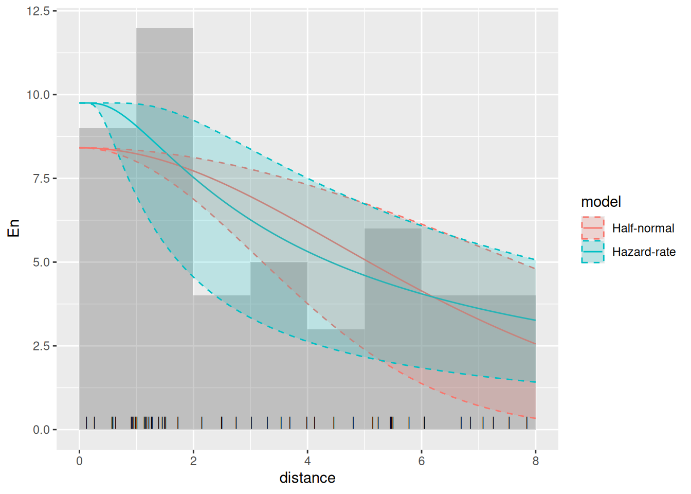
Plot with the 95% credible intervals (without taking the count rescaling into account)

ggplot(data.frame(mexdolphin$points)) +
  geom_histogram(aes(x = distance), breaks = seq(0, 8, length.out = 9), alpha = 0.3) +
  geom_point(aes(x = distance), y = 0.2, shape = "|", size = 3) +
  geom_line(data = dlines, aes(x = distance, y = En, group = model, col = model)) +
  geom_ribbon(
    data = dlines, aes(x = distance, ymin = En.lower, ymax = En.upper, group = model, col = model, fill = model),
    alpha = 0.2, lty = 2
  )

LGCPs - Distance sampling

David Borchers and Finn Lindgren