LGCPs - An example in two dimensions • inlabru

Introduction

For this vignette we are going to be working with a dataset obtained from the R package spatstat. We will set up a two-dimensional LGCP to estimate Gorilla abundance.

Setting things up

Load libraries

library(inlabru)
library(INLA)
library(mgcv)
library(ggplot2)
bru_safe_sp(force = TRUE)

Get the data

For the next few practicals we are going to be working with a dataset obtained from the R package spatstat, which contains the locations of 647 gorilla nests. We load the dataset in sp format like this:

gorillas <- gorillas_sp()
#> Loading required namespace: terra

This dataset is a list containing a number of R objects, including the locations of the nests, the boundary of the survey area and an INLA mesh - see help(gorillas) for details. Extract the the objects we need from the list, into other objects, so that we don’t have to keep typing ‘gorillas$’:

nests <- gorillas$nests
mesh <- gorillas$mesh
boundary <- gorillas$boundary

Plot the points (the nests).

ggplot() +
  geom_fm(data = mesh) +
  gg(nests) +
  gg(boundary, fill = "red", alpha = 0.2) +
  ggtitle("Points")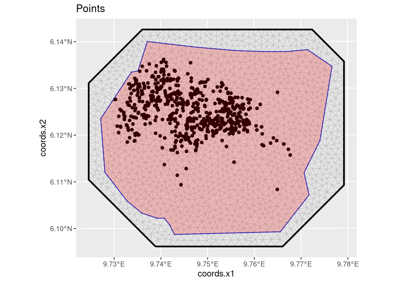

Fiting the model

Fit an LGCP model to the locations of the gorilla nests, predict on the survey region, and produce a plot of the estimated density - which should look like the plot shown below.

Recall that the steps to specifying, fitting and predicting are:

Specify a model, comprising (for 2D models) coordinates on the left of ~ and an SPDE + Intercept(1) on the right. Please use the SPDE prior specification stated below.
Call lgcp( ), passing it (with 2D models) the model components, the SpatialPointsDataFrame containing the observed points and the SpatialPolygonsDataFrame defining the survey boundary using the samplers argument.
Call predict( ), passing it the fitted model from 2., locations at which to predict and an appropriate predictor specification. The locations at which to predict can be a SpatialPixelsDataFrame covering the mesh, obtained by calling fm_pixels(mesh, format = "sp").

matern <- inla.spde2.pcmatern(
  mesh,
  prior.sigma = c(0.1, 0.01),
  prior.range = c(5, 0.01)
)

cmp <- coordinates ~
  mySmooth(coordinates, model = matern) +
  Intercept(1)

fit <- lgcp(cmp, nests, samplers = boundary, domain = list(coordinates = mesh))

Predicting intensity

You should get a plot like that below (the command below assumes that the prediction is in an object called lambda):

pred <- predict(
  fit,
  fm_pixels(mesh, mask = boundary, format = "sp"),
  ~ data.frame(
    lambda = exp(mySmooth + Intercept),
    loglambda = mySmooth + Intercept
  )
)

pl1 <- ggplot() +
  gg(pred$lambda) +
  gg(boundary) +
  ggtitle("LGCP fit to Points", subtitle = "(Response Scale)")

pl2 <- ggplot() +
  gg(pred$loglambda) +
  gg(boundary, alpha = 0) +
  ggtitle("LGCP fit to Points", subtitle = "(Linear Predictor Scale)")

multiplot(pl1, pl2, cols = 2)

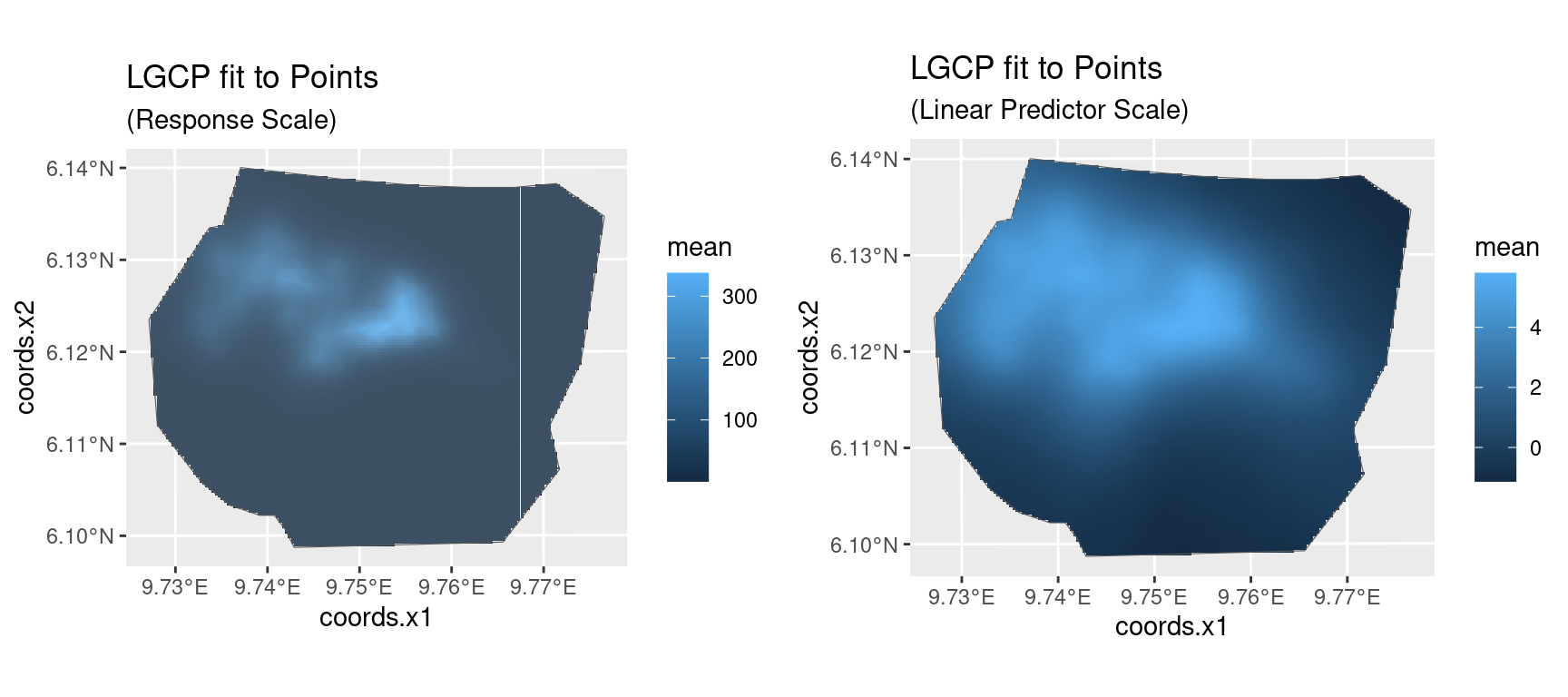
You can plot the median, lower 95% and upper 95% density surfaces as follows (assuming that the predicted intensity is in object lambda).

ggplot() +
  gg(cbind(pred$lambda, data.frame(property = "q0.500")), aes(fill = median)) +
  gg(cbind(pred$lambda, data.frame(property = "q0.025")), aes(fill = q0.025)) +
  gg(cbind(pred$lambda, data.frame(property = "q0.975")), aes(fill = q0.975)) +
  coord_equal() +
  facet_wrap(~property)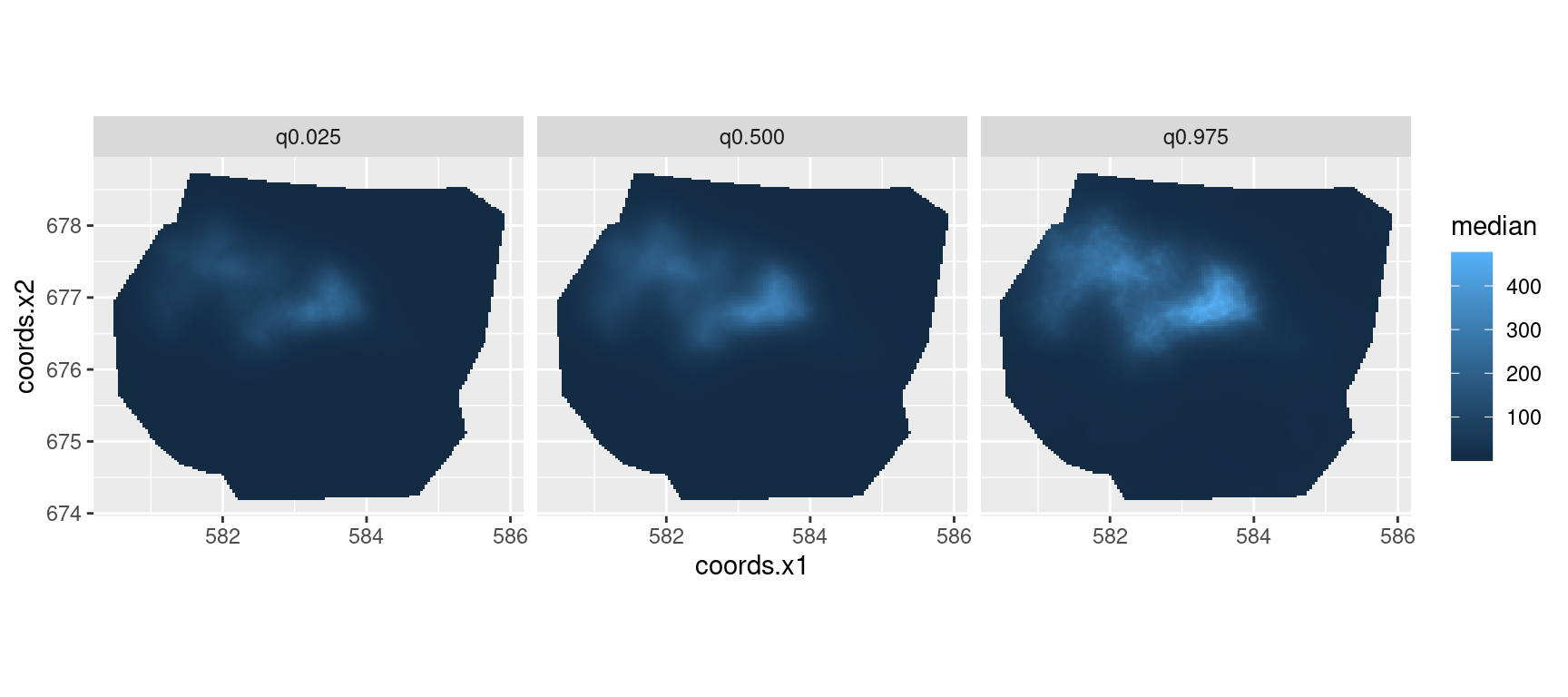

SPDE parameters

Plot the SPDE parameter and fixed effect parameter posteriors.

int.plot <- plot(fit, "Intercept")
spde.range <- spde.posterior(fit, "mySmooth", what = "range")
spde.logvar <- spde.posterior(fit, "mySmooth", what = "log.variance")
range.plot <- plot(spde.range)
var.plot <- plot(spde.logvar)

multiplot(range.plot, var.plot, int.plot)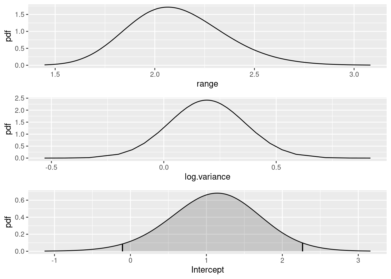

Look at the correlation function if you want to:

corplot <- plot(spde.posterior(fit, "mySmooth", what = "matern.correlation"))
covplot <- plot(spde.posterior(fit, "mySmooth", what = "matern.covariance"))
multiplot(covplot, corplot)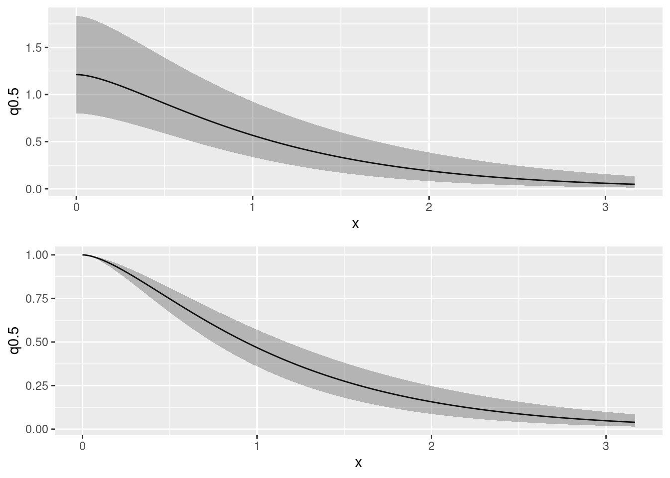

Estimating Abundance

Finally, estimate abundance using the predict function. As a first step we need an estimate for the integrated lambda. The integration weight values are contained in the fm_int() output.

Lambda <- predict(
  fit,
  fm_int(mesh, boundary),
  ~ sum(weight * exp(mySmooth + Intercept))
)
Lambda
#>      mean       sd   q0.025     q0.5   q0.975   median sd.mc_std_err
#> 1 668.325 27.56141 620.7193 664.5534 722.2724 664.5534      1.764344
#>   mean.mc_std_err
#> 1         3.10901

Given some generous interval boundaries (500, 800) for lambda we can estimate the posterior abundance distribution via

Nest <- predict(
  fit, fm_int(mesh, boundary),
  ~ data.frame(
    N = 500:800,
    dpois(500:800,
      lambda = sum(weight * exp(mySmooth + Intercept))
    )
  )
)

Get its quantiles via

inla.qmarginal(c(0.025, 0.5, 0.975), marginal = list(x = Nest$N, y = Nest$mean))
#> [1] 597.7930 665.4090 734.9173

… the mean via

inla.emarginal(identity, marginal = list(x = Nest$N, y = Nest$mean))
#> [1] 665.6916

and plot posteriors:

Nest$plugin_estimate <- dpois(Nest$N, lambda = Lambda$mean)
ggplot(data = Nest) +
  geom_line(aes(x = N, y = mean, colour = "Posterior")) +
  geom_line(aes(x = N, y = plugin_estimate, colour = "Plugin"))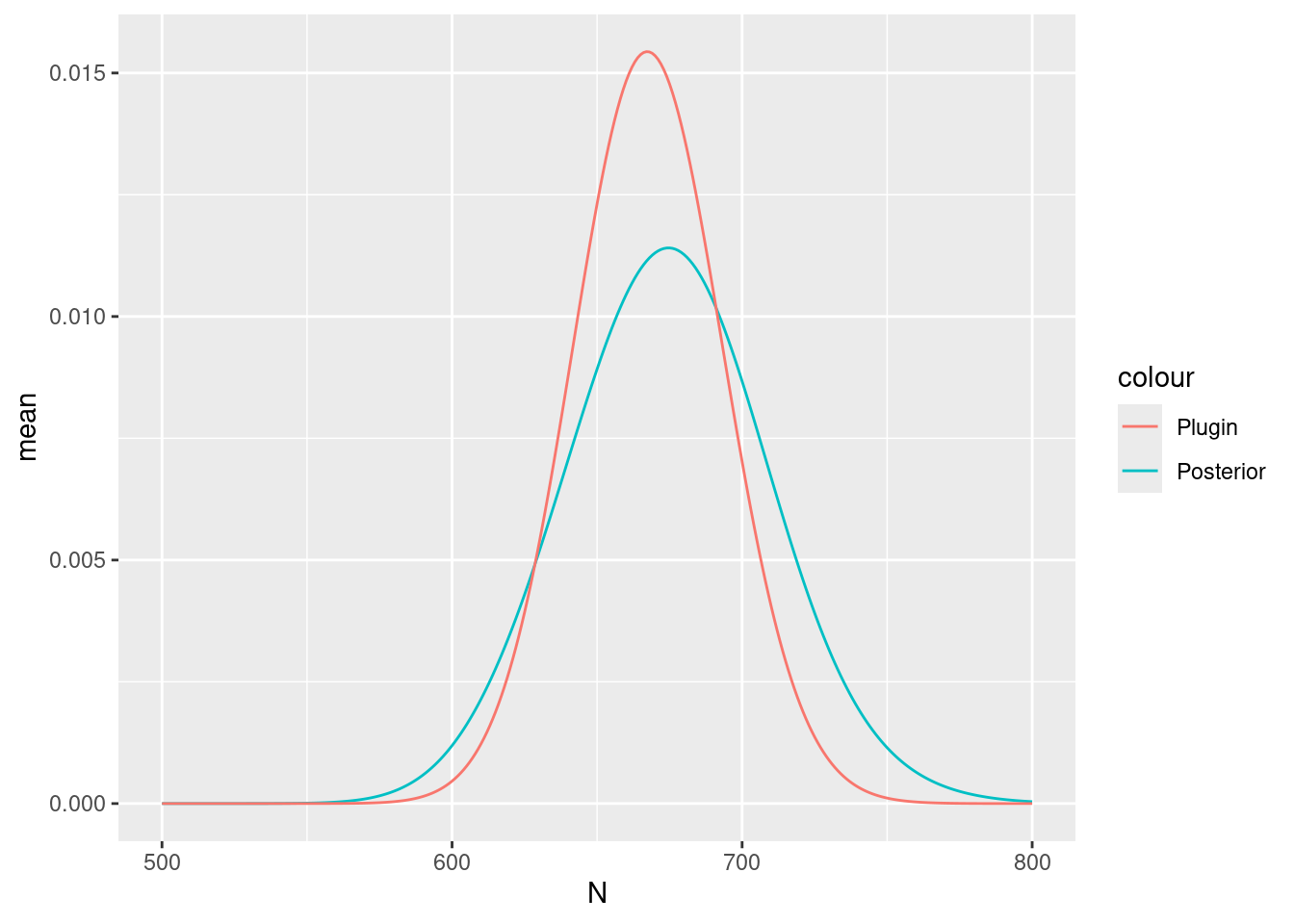

The true number of nests in 647; the mean and median of the posterior distribution of abundance should be close to this if you have not done anything wrong!

LGCPs - An example in two dimensions

David Borchers and Finn Lindgren