LGCPs - Plot sampling

David Borchers and Finn Lindgren

Generated on 2025-06-16

Introduction

This practical demonstrates use of the samplers argument in lgcp, which you need to use when you have observed points from only a sample of plots in the survey region.

Setting things up

Load libraries

library(inlabru)
library(INLA)
library(mgcv)
library(ggplot2)

Get the data

data(gorillas_sf, package = "inlabru")

This dataset is a list (see help(gorillas_sf) for details. Extract the the objects you need from the list, for convenience:

nests <- gorillas_sf$nests
mesh <- gorillas_sf$mesh
boundary <- gorillas_sf$boundary
gcov <- gorillas_sf_gcov()
#> Loading required namespace: terra

The gorillas_sf data also contains a plot sample subset which covers 60% of the survey region.

sample <- gorillas_sf$plotsample

plotdets <- ggplot() +
  gg(boundary) +
  gg(sample$plots) +
  gg(sample$nests, pch = "+", cex = 4, color = "red") +
  geom_text(aes(
    label = sample$counts$count,
    x = sf::st_coordinates(sample$counts)[, 1],
    y = sf::st_coordinates(sample$counts)[, 2]
  )) +
  labs(x = "Easting", y = "Northing")
plot(plotdets)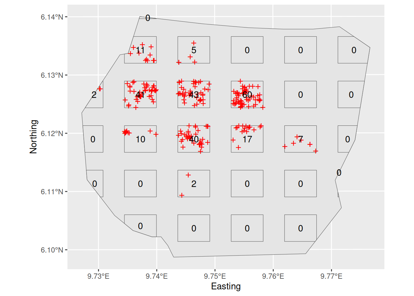

On this plot survey, only points within the rectangles are detected, but it is also informative to plot all the points here (which if it was a real plot survey you could not do, because you would not have seen them all).

plotwithall <- ggplot() +
  gg(boundary) +
  gg(sample$plots) +
  gg(nests, pch = "+", cex = 4, color = "blue") +
  geom_text(aes(
    label = sample$counts$count,
    x = sf::st_coordinates(sample$counts)[, 1],
    y = sf::st_coordinates(sample$counts)[, 2]
  )) +
  gg(sample$nests, pch = "+", cex = 4, color = "red") +
  labs(x = "Easting", y = "Northing")
plot(plotwithall)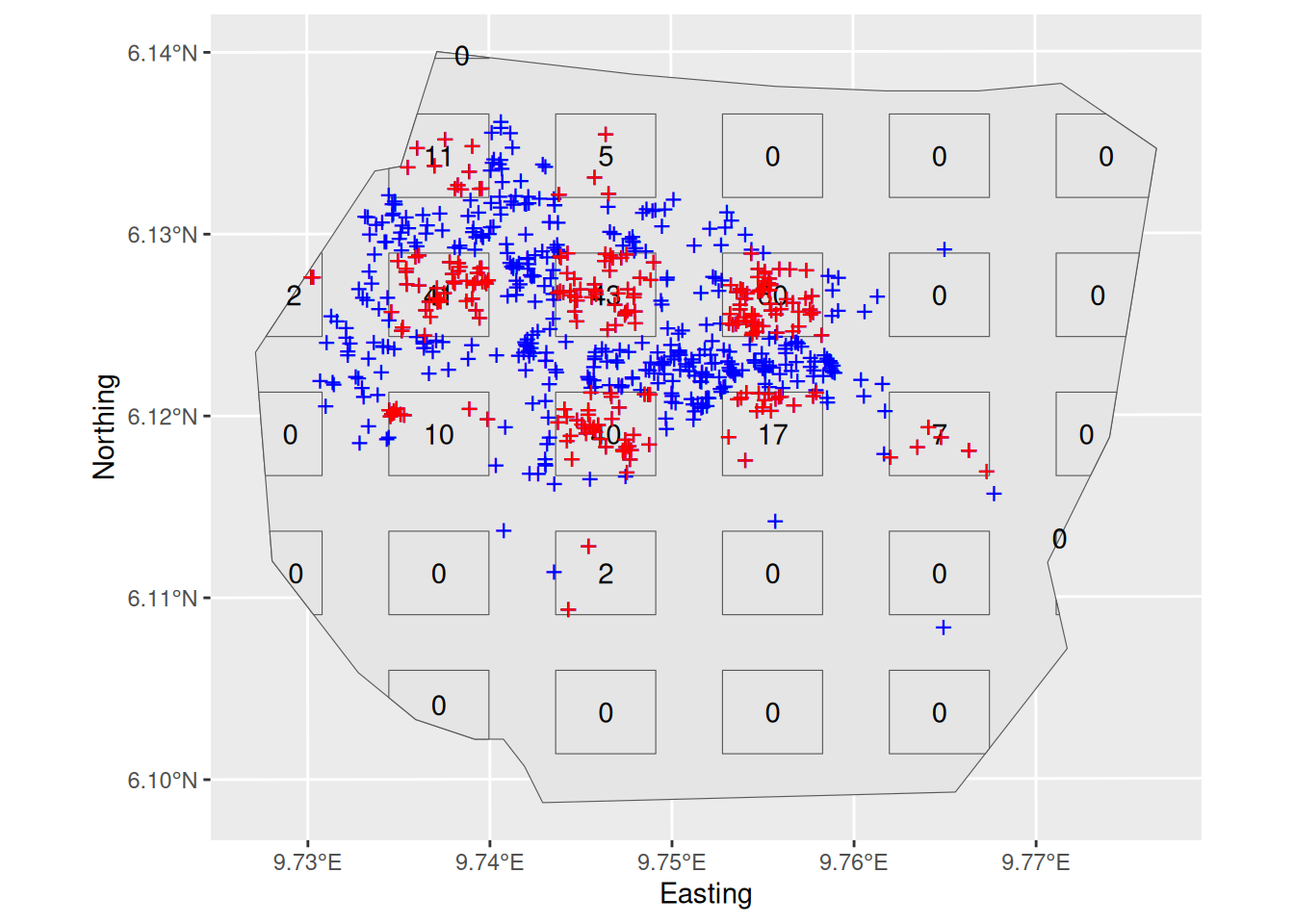

Inference

The observed nest locations are in the sf sample$nests, and the plots are in the sf sample$plots. Again, we are using the following SPDE setup:

matern <- inla.spde2.pcmatern(mesh,
  prior.sigma = c(0.1, 0.01),
  prior.range = c(0.05, 0.01)
)

Fit an LGCP model with SPDE only to these data by using the samplers= argument of the function lgcp( ):

cmp <- geometry ~ my.spde(geometry, model = matern)

fit <- lgcp(cmp,
  sample$nests,
  samplers = sample$plots,
  domain = list(geometry = mesh)
)

Plot the density surface from your fitted model

pxl <- fm_pixels(mesh, mask = boundary)
lambda.sample <- predict(fit, pxl, ~ exp(my.spde + Intercept))

lambda.sample.plot <- ggplot() +
  gg(lambda.sample, geom = "tile") +
  gg(sample$plots, alpha = 0) +
  gg(boundary, col = "yellow", alpha = 0)

lambda.sample.plot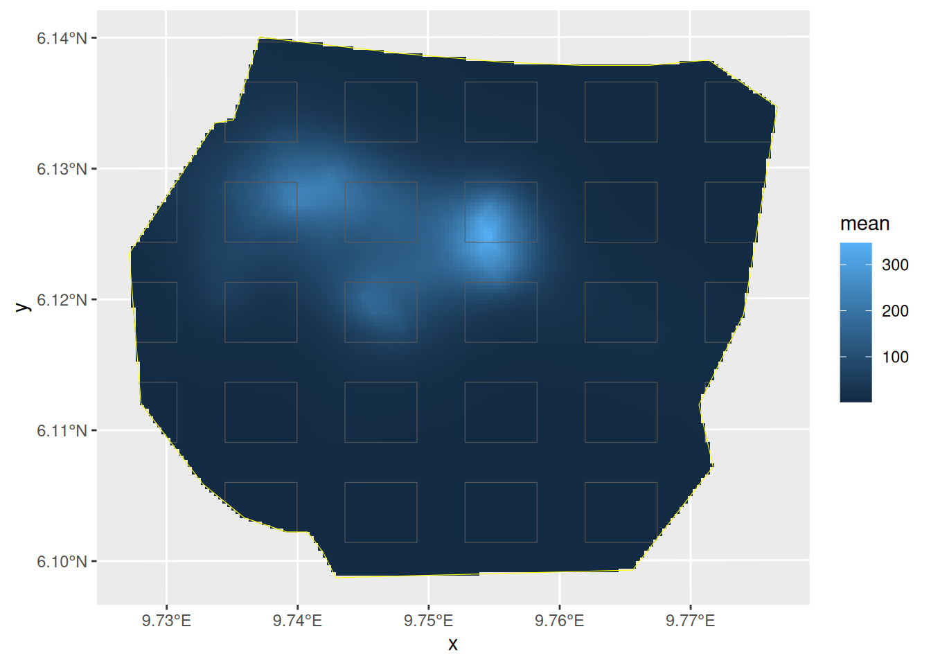

Estimate the integrated intensity lambda. We compute both the overall integrated intensity, representative of an imagined new realisation of the point process, and the conditional expectation that takes the actually observed nests into account, by recognising that we have complete information in the surveyed plots.

Lambda <- predict(
  fit,
  fm_int(mesh, boundary),
  ~ sum(weight * exp(my.spde + Intercept))
)
Lambda.empirical <- predict(
  fit,
  rbind(
    cbind(fm_int(mesh, boundary), data.frame(all = TRUE)),
    cbind(fm_int(mesh, sample$plots), data.frame(all = FALSE))
  ),
  ~ (sum(weight * exp(my.spde + Intercept) * all) -
    sum(weight * exp(my.spde + Intercept) * !all) +
    nrow(sample$nests))
)
rbind(
  Lambda,
  Lambda.empirical
)

Fit the same model to the full dataset (the points in gorillas_sf$nests), or get your previous fit, if you kept it. Plot the intensity surface and estimate the integrated intensity

fit.all <- lgcp(cmp, nests,
  samplers = boundary,
  domain = list(geometry = mesh)
)
lambda.all <- predict(fit.all, pxl, ~ exp(my.spde + Intercept))
Lambda.all <- predict(
  fit.all,
  fm_int(mesh, boundary),
  ~ sum(weight * exp(my.spde + Intercept))
)

Your plot should look like this:

The values Lambda.empirical, Lambda, and Lambda.all should be close to each other if the plot samples gave sufficient information for the overall prediction:

rbind(
  Plots = Lambda,
  PlotsEmp = Lambda.empirical,
  All = Lambda.all,
  AllEmp = c(
    nrow(gorillas_sf$nests),
    0,
    rep(nrow(gorillas_sf$nests), 3),
    rep(NA, 3)
  )
)
#>              mean       sd   q0.025     q0.5   q0.975   median sd.mc_std_err
#> Plots    656.3640 59.42197 548.3281 654.8737 763.9415 654.8737      5.171820
#> PlotsEmp 642.6092 38.32410 578.9110 644.7476 719.6881 644.7476      2.323733
#> All      675.7708 25.65538 632.8818 676.1423 714.5690 676.1423      1.742837
#> AllEmp   647.0000  0.00000 647.0000 647.0000 647.0000       NA            NA
#>          mean.mc_std_err
#> Plots           6.976561
#> PlotsEmp        4.297156
#> All             2.914106
#> AllEmp                NA

Now, let’s compare the results

library(patchwork)
lambda.sample.plot + lambda.all.plot +
  plot_layout(guides = "collect") &
  theme(legend.position = "left") &
  scale_fill_continuous(limits = range(c(0, 340)))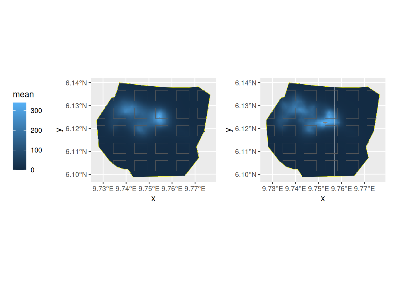

Do you understand the reason for the differences in the posteriors of the abundance estimates?