Geoms for sp Spatial objects

Methods for plotting sp spatial objects with ggplot2.

Usage

# S3 method for class 'SpatialPoints'
gg(data, mapping = NULL, crs = NULL, ...)

# S3 method for class 'SpatialLines'
gg(data, mapping = NULL, crs = NULL, ...)

# S3 method for class 'SpatialPolygons'
gg(data, mapping = NULL, crs = NULL, ...)

# S3 method for class 'SpatialGridDataFrame'
gg(data, ...)

# S3 method for class 'SpatialPixelsDataFrame'
gg(data, mapping = NULL, crs = NULL, mask = NULL, ...)

# S3 method for class 'SpatialPixels'
gg(data, ...)

Arguments

data

A Spatial* object.

mapping

Aesthetic mappings created by aes used to update the default mapping. Uness specified otherwise below, the default mapping is

ggplot2::aes(
  x = .data[[sp::coordnames(data)[1]]],
  y = .data[[sp::coordnames(data)[2]]]
)

crs

A sp::CRS object defining the coordinate system to project the data to before plotting.

...

Arguments passed on to geom_*.

mask

A sp::SpatialPolygons object defining the region that is plotted.

Value

A geom_point, geom_segment, geom_sf, geom_tile, or a list of ggplot geomes

Functions

gg(SpatialPoints): Geom for SpatialPoints objects. This function coerces the SpatialPoints into a data.frame and uses geom_point to plot the points. Requires the ggplot2 package.
gg(SpatialLines): Geom for SpatialLines objects.

Extracts start and end points of the lines and calls geom_segment to plot lines between them.

mapping: Aesthetic mappings created by ggplot2::aes or ggplot2::aes_ used to update the default mapping. The default mapping is
```
ggplot2::aes(
  x = .data[[sp::coordnames(data)[1]]],
  y = .data[[sp::coordnames(data)[2]]],
  xend = .data[[paste0("end.", sp::coordnames(data)[1])]],
  yend = .data[[paste0("end.", sp::coordnames(data)[2])]])
```
gg(SpatialPolygons): Geom for SpatialPolygons objects. Uses the ggplot2::fortify() function to turn the SpatialPolygons objects into a data.frame. Then calls geom_polygon to plot the polygons.

Unless specified by the user, the argument alpha = 0.2 (alpha level for polygon filling) is added.

Up to version 2.10.0, the ggpolypath package was used to ensure proper plotting for polygons, since the ggplot2::geom_polygon function doesn't always handle geometries with holes properly. After 2.10.0, the object is converted to sf format and passed on to gg.sf() instead, as ggplot2 version 3.4.4 deprecated the internally used ggplot2::fortify() method for SpatialPolygons/DataFrame objects.
gg(SpatialGridDataFrame): Geom for SpatialGridDataFrame objects

Coerces input SpatialGridDataFrame to SpatialPixelsDataFrame and calls gg.SpatialPixelsDataFrame() to plot it.
gg(SpatialPixelsDataFrame): Geom for SpatialPixelsDataFrame objects.

Coerces SpatialPixelsDataFrame input to data.frame and uses geom_tile to plot it.

mapping: Aesthetic mappings created by aes used to update the default mapping. The default mapping is
```
ggplot2::aes(
  x = .data[[sp::coordnames(data)[1]]],
  y = .data[[sp::coordnames(data)[2]]],
  fill = .data[[names(data)[[1]]]]
)
```
gg(SpatialPixels): Geom for SpatialPixels objects

Converts the input to SpatialPoints and calls [gg.SpatialPoints()` to plot it.

Examples

# \donttest{
if (require("ggplot2", quietly = TRUE) &&
  bru_safe_terra(quietly = TRUE) &&
  bru_safe_sp() &&
  require("sp")) {
  # Load Gorilla data

  gorillas <- inlabru::gorillas_sf

  gcov <- gorillas_sf_gcov()
  elev <- terra::as.data.frame(gcov$elevation, xy = TRUE)
  elev <- sf::as_Spatial(sf::st_as_sf(elev, coords = c("x", "y")))

  # Turn elevation covariate into SpatialGridDataFrame
  elev <- sp::SpatialPixelsDataFrame(elev, data = as.data.frame(elev))

  # Plot Gorilla elevation covariate provided as SpatialPixelsDataFrame.
  # The same syntax applies to SpatialGridDataFrame objects.

  ggplot() +
    gg(elev)

  # Add Gorilla survey boundary and nest sightings

  ggplot() +
    gg(elev) +
    gg(gorillas$boundary, alpha = 0.0, col = "red") +
    gg(gorillas$nests)

  # Load pantropical dolphin data

  mexdolphin <- inlabru::mexdolphin_sp()

  # Plot the pantropical survey boundary, ship transects, and dolphin
  # sightings

  ggplot() +
    gg(mexdolphin$ppoly) + # survey boundary as SpatialPolygon
    gg(mexdolphin$samplers) + # ship transects as SpatialLines
    gg(mexdolphin$points) # dolphin sightings as SpatialPoints

  # Change color

  ggplot() +
    gg(mexdolphin$ppoly, color = "green") + # survey boundary; SpatialPolygon
    gg(mexdolphin$samplers, color = "red") + # ship transects; SpatialLines
    gg(mexdolphin$points, color = "blue") # dolphin sightings; SpatialPoints


  # Visualize data annotations: line width by segment number

  names(mexdolphin$samplers) # 'seg' holds the segment number
  ggplot() +
    gg(mexdolphin$samplers, aes(color = seg))

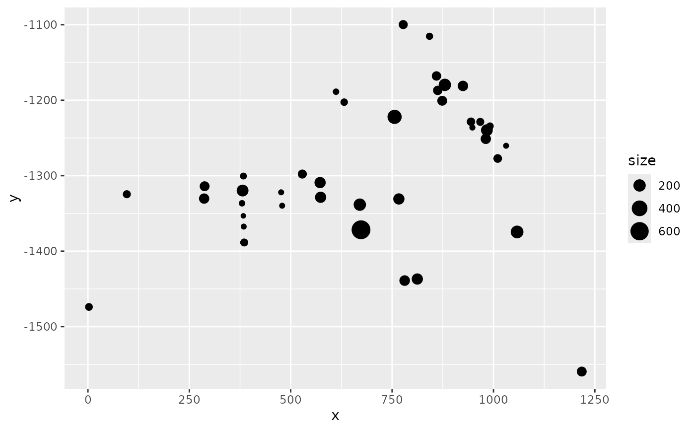
  # Visualize data annotations: point size by dolphin group size

  names(mexdolphin$points) # 'size' holds the group size
  ggplot() +
    gg(mexdolphin$points, aes(size = size))
}
#> Loading required package: sp

# }

if (require("ggplot2", quietly = TRUE) &&
  bru_safe_terra(quietly = TRUE) &&
  bru_safe_sp()) {
  # Load Gorilla data

  gcov <- gorillas_sf_gcov()
  elev <- terra::as.data.frame(gcov$elevation, xy = TRUE)
  pxl <- sf::as_Spatial(sf::st_as_sf(elev, coords = c("x", "y")))

  # Turn elevation covariate into SpatialPixels
  pxl <- sp::SpatialPixels(pxl)

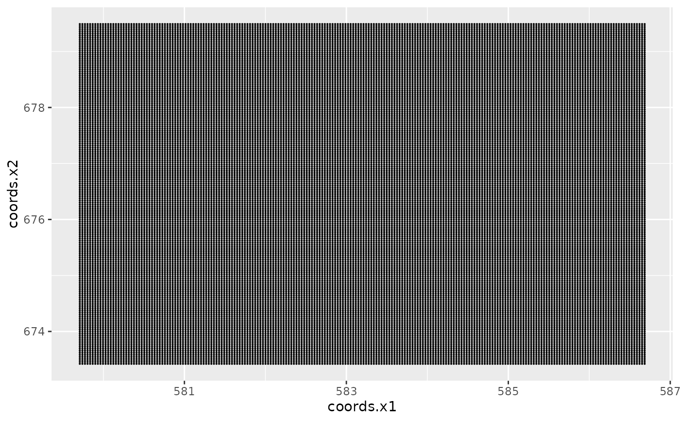
  # Plot the pixel centers
  ggplot() +
    gg(pxl, size = 0.1)
}

Usage

Arguments

Value

Functions

See also

Examples