Prediction from fitted bru model — predict.bru • inlabru

Takes a fitted bru object produced by the function bru() and produces predictions given a new set of values for the model covariates or the original values used for the model fit. The predictions can be based on any R expression that is valid given these values/covariates and the joint posterior of the estimated random effects.

Usage

# S3 method for bru
predict(
  object,
  newdata = NULL,
  formula = NULL,
  n.samples = 100,
  seed = 0L,
  probs = c(0.025, 0.5, 0.975),
  num.threads = NULL,
  include = NULL,
  exclude = NULL,
  used = NULL,
  drop = FALSE,
  ...,
  data = deprecated()
)

Arguments

object: An object obtained by calling bru() or lgcp().
newdata: A data.frame or SpatialPointsDataFrame of covariates needed for the prediction.
formula: A formula where the right hand side defines an R expression to evaluate for each generated sample. If NULL, the latent and hyperparameter states are returned as named list elements. See Details for more information.
n.samples: Integer setting the number of samples to draw in order to calculate the posterior statistics. The default is rather low but provides a quick approximate result.
seed: Random number generator seed passed on to inla.posterior.sample
probs: A numeric vector of probabilities with values in [0, 1], passed to stats::quantile
num.threads: Specification of desired number of threads for parallel computations. Default NULL, leaves it up to INLA. When seed != 0, overridden to "1:1"
include: Character vector of component labels that are needed by the predictor expression; Default: the result of [all.vars()] on the predictor expression, unless the expression is not ".", in which case include=NULL, to include all components that are not explicitly excluded. The bru_used() methods are used to extract the variable names, followed by removal of non-component names when the components are available.
exclude: Character vector of component labels that are not used by the predictor expression. The exclusion list is applied to the list as determined by the include parameter; Default: NULL (do not remove any components from the inclusion list)
used: Either NULL or a bru_used() object, overriding include and exclude. Default NULL
drop: logical; If keep=FALSE, newdata is a Spatial*DataFrame, and the prediciton summary has the same number of rows as newdata, then the output is a Spatial*DataFrame object. Default FALSE.
...: Additional arguments passed on to inla.posterior.sample()
data: Use newdata instead.

Value

a data.frame, sf, or Spatial* object with predicted mean values and other summary statistics attached. Non-S4 object outputs have the class "bru_prediction" added at the front of the class list.

Details

Mean value predictions are accompanied by the standard errors, upper and lower 2.5% quantiles, the median, variance, coefficient of variation as well as the variance and minimum and maximum sample value drawn in course of estimating the statistics.

Internally, this method calls generate.bru() in order to draw samples from the model.

In addition to the component names (that give the effect of each component evaluated for the input data), the suffix _latent variable name can be used to directly access the latent state for a component, and the suffix function _eval can be used to evaluate a component at other input values than the expressions defined in the component definition itself, e.g. field_eval(cbind(x, y)) for a component that was defined with field(coordinates, ...) (see also component_eval()).

For "iid" models with mapper = bru_mapper_index(n), rnorm() is used to generate new realisations for indices greater than n.

Examples

# \donttest{
if (bru_safe_inla(multicore = FALSE) &&
    bru_safe_sp() &&
    require("sp") &&
    require("sn", quietly = TRUE) &&
    require("ggplot2", quietly = TRUE)) {

  # Load the Gorilla data

  data(gorillas, package = "inlabru")

  # Plot the Gorilla nests, the mesh and the survey boundary

  ggplot() +
    gg(gorillas$mesh) +
    gg(gorillas$nests) +
    gg(gorillas$boundary)

  # Define SPDE prior

  matern <- INLA::inla.spde2.pcmatern(gorillas$mesh,
    prior.sigma = c(0.1, 0.01),
    prior.range = c(0.01, 0.01)
  )

  # Define domain of the LGCP as well as the model components (spatial SPDE effect and Intercept)

  cmp <- coordinates ~ mySmooth(main = coordinates, model = matern) + Intercept(1)

  # Fit the model, with "eb" instead of full Bayes
  fit <- lgcp(cmp, gorillas$nests,
    samplers = gorillas$boundary,
    domain = list(coordinates = gorillas$mesh),
    options = list(control.inla = list(int.strategy = "eb"))
  )

  # Once we obtain a fitted model the predict function can serve various purposes.
  # The most basic one is to determine posterior statistics of a univariate
  # random variable in the model, e.g. the intercept

  icpt <- predict(fit, NULL, ~ c(Intercept = Intercept_latent))
  plot(icpt)

  # The formula argument can take any expression that is valid within the model, for
  # instance a non-linear transformation of a random variable

  exp.icpt <- predict(fit, NULL, ~ c(
    "Intercept" = Intercept_latent,
    "exp(Intercept)" = exp(Intercept_latent)
  ))
  plot(exp.icpt, bar = TRUE)

  # The intercept is special in the sense that it does not depend on other variables
  # or covariates. However, this is not true for the smooth spatial effects 'mySmooth'.
  # In order to predict 'mySmooth' we have to define where (in space) to predict. For
  # this purpose, the second argument of the predict function can take \code{data.frame}
  # objects as well as Spatial objects. For instance, we might want to predict
  # 'mySmooth' at the locations of the mesh vertices. Using

  vrt <- fm_vertices(gorillas$mesh, format = "sp")

  # we obtain these vertices as a SpatialPointsDataFrame

  ggplot() +
    gg(gorillas$mesh) +
    gg(vrt, color = "red")

  # Predicting 'mySmooth' at these locations works as follows

  mySmooth <- predict(fit, vrt, ~mySmooth)

  # Note that just like the input also the output will be a SpatialPointsDataFrame
  # and that the predicted statistics are simply added as columns

  class(mySmooth)
  head(vrt)
  head(mySmooth)

  # Plotting the mean, for instance, at the mesh node is straight forward

  ggplot() +
    gg(gorillas$mesh) +
    gg(mySmooth, aes(color = mean), size = 3)

  # However, we are often interested in a spatial field and thus a linear interpolation,
  # which can be achieved by using the gg mechanism for meshes

  ggplot() +
    gg(gorillas$mesh, color = mySmooth$mean)

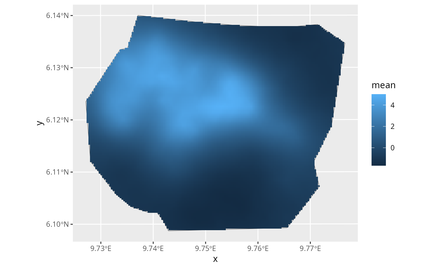
  # Alternatively, we can predict the spatial field at a grid of locations, e.g. a
  # SpatialPixels object covering the mesh

  pxl <- fm_pixels(gorillas$mesh, format = "sp")
  mySmooth2 <- predict(fit, pxl, ~mySmooth)

  # This will give us a SpatialPixelDataFrame with the columns we are looking for

  head(mySmooth2)
  ggplot() +
    gg(mySmooth2)
}
#> Current num.threads is '1:1'.
#> No num.threads change needed.

# }