Make hierarchical mesh basis functions

Construct hierarchical basis functions. This is highly experimental and may change or be removed in future versions.

Usage

make_hierarchical_mesh_basis(mesh, forward = TRUE, method = NULL, alpha = 1)

inla.spde2.pcmatern_B(mesh, ..., B)

Arguments

mesh: A fmesher object.
forward: logical; if TRUE (default), the basis functions are constructed in forward order; otherwise in reverse order.
method: Character; one of "laplace" (default), "graphdistance" or "graphlaplace". The method used to construct the basis functions. See Details.
alpha: Numeric; only used if method = "laplace". The approximate Laplacian power used to construct the basis functions. Default is (1 + fm_manifold_dim(mesh)) / 2, which gives an approximately linear function along the shortest path. Must be in the range [1, 2]. See Details.

Value

A sparse matrix of class dgCMatrix, where each column corresponds to a basis function.

Details

The hierarchical basis functions are constructed by iteratively adding basis functions centered at the point furthest away from the previously added basis functions. The radius of each basis function is equal to the distance to the previously added basis functions at the time of addition. Three methods are available to construct the basis functions:

laplace: The basis functions are constructed using a combination of two operators, the Laplacian and the squared Laplacian (the biharmonic operator). This approximates the Laplacian raised to the power alpha. The default value for alpha gives an approximately linear function along the shortest path.one based on the standard FEM stiffness matrix, and one based on the graph Laplacian. The alpha parameter controls the weight between the two operators, with alpha = 1 using only the Laplacian and alpha = 2 using only the squared Laplacian.
graphdistance: The basis functions are constructed using a simple neighbour distance-based approach, where the basis function value decreases by equal amounts for each traversed edge.
graphlaplace: The basis functions are constructed using the graph Laplacian only.

Functions

inla.spde2.pcmatern_B(): Construct a pcmatern model with basis change

Examples

m <- fmesher::fmexample$mesh
B <- make_hierarchical_mesh_basis(m, method = "laplace2", alpha = 1.5)

# \donttest{
m <- fmesher::fm_subdivide(fmesher::fmexample$mesh, 1)
B <- list()
for (method in c(
  "laplace", "laplace2",
  "graphdistance",
  "graphlaplace", "graphlaplace2"
)) {
  B[[method]] <- make_hierarchical_mesh_basis(
    m,
    method = method, alpha = 1.5
  )
}
if (require("ggplot2") && require("patchwork")) {
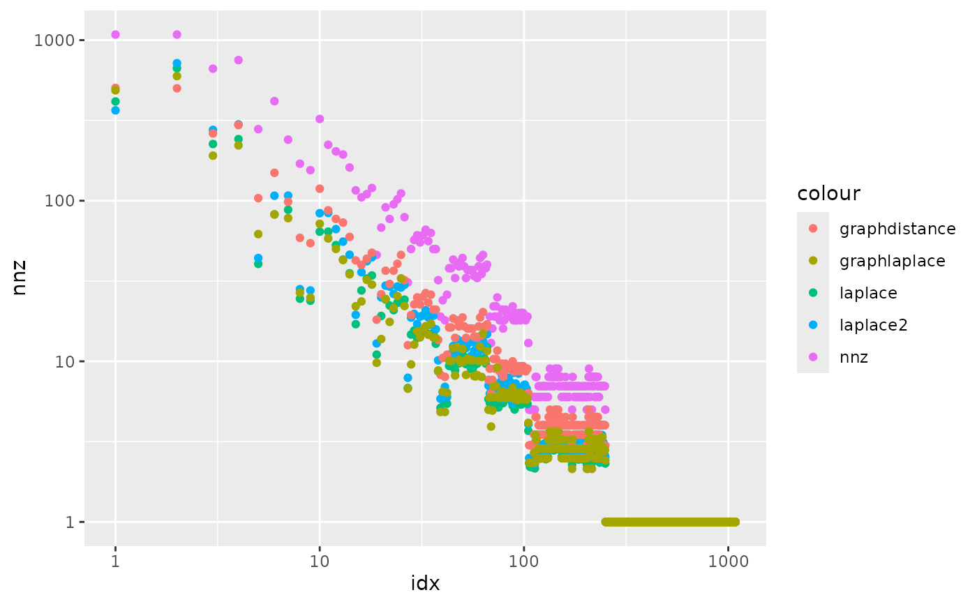
  print(
    ggplot(
      data =
        data.frame(
          idx = seq_len(ncol(B$laplace)),
          nnz = as.vector(Matrix::colSums(0 != B$laplace)),
          laplace = as.vector(Matrix::colSums(B$laplace)),
          laplace2 = as.vector(Matrix::colSums(B$laplace2)),
          distance = as.vector(Matrix::colSums(B$graphdistance)),
          graph = as.vector(Matrix::colSums(B$graphlaplace)),
          graph2 = as.vector(Matrix::colSums(B$graphlaplace2))
        )
    ) +
      geom_point(aes(x = idx, y = nnz, color = "nnz")) +
      geom_point(aes(x = idx, y = laplace, color = "laplace")) +
      geom_point(aes(x = idx, y = laplace2, color = "laplace2")) +
      geom_point(aes(x = idx, y = distance, color = "graphdistance")) +
      geom_point(aes(x = idx, y = graph, color = "graphlaplace")) +
      scale_y_log10() +
      scale_x_log10()
  )

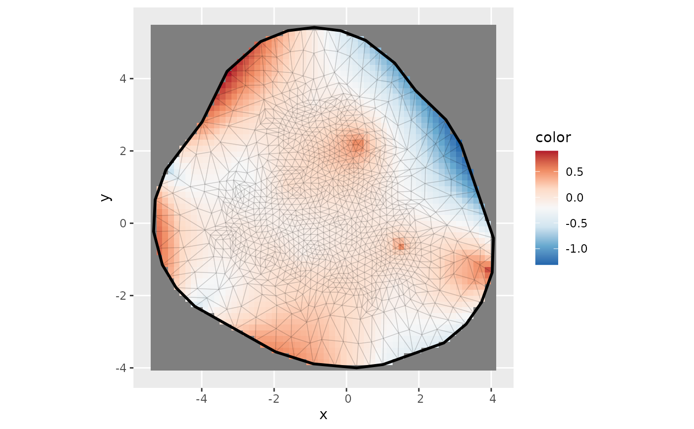
  idx <- seq_len(fm_dof(m))
  idx <- seq_len(10)
  method <- "laplace"
  theta <- qr.solve(B[[method]][, idx, drop = FALSE], m$loc[, 1])
  print(
    ggplot() +
      gg(m,
        col = B[[method]][, idx, drop = FALSE] %*% theta - m$loc[, 1],
        nx = 60, ny = 60
      ) +
      geom_fm(data = m, color = ggplot2::alpha("black", 0.1), alpha = 0) +
      scale_fill_distiller(palette = "RdBu")
  )

  ev <- fm_evaluator(m, dims = c(60, 60))
  df <- NULL
  for (method in c(
    "laplace", "laplace2",
    "graphdistance",
    "graphlaplace", "graphlaplace2"
  )) {
    fun_cumulative <- 1e-16
    for (k in 1:28) {
      fun_orig <- as.vector(B[[method]][, k, drop = FALSE])
      fun_cumulative <- fun_cumulative + fun_orig
      fun_norm <- fun_orig / fun_cumulative
      df <- rbind(
        df,
        data.frame(
          x = ev$lattice$loc[, 1],
          y = ev$lattice$loc[, 2],
          orig = as.vector(fm_evaluate(ev, fun_orig)),
          norm = as.vector(fm_evaluate(ev, fun_norm)),
          index = k,
          fun = paste0(
            "fun",
            formatC(k, width = 2, format = "d", flag = "0")
          ),
          method = method
        )
      )
    }
  }
  df$norm[df$fun == "fun01"] <- NA
  df$orig[df$orig == 0] <- NA
  df$norm[df$norm == 0] <- NA
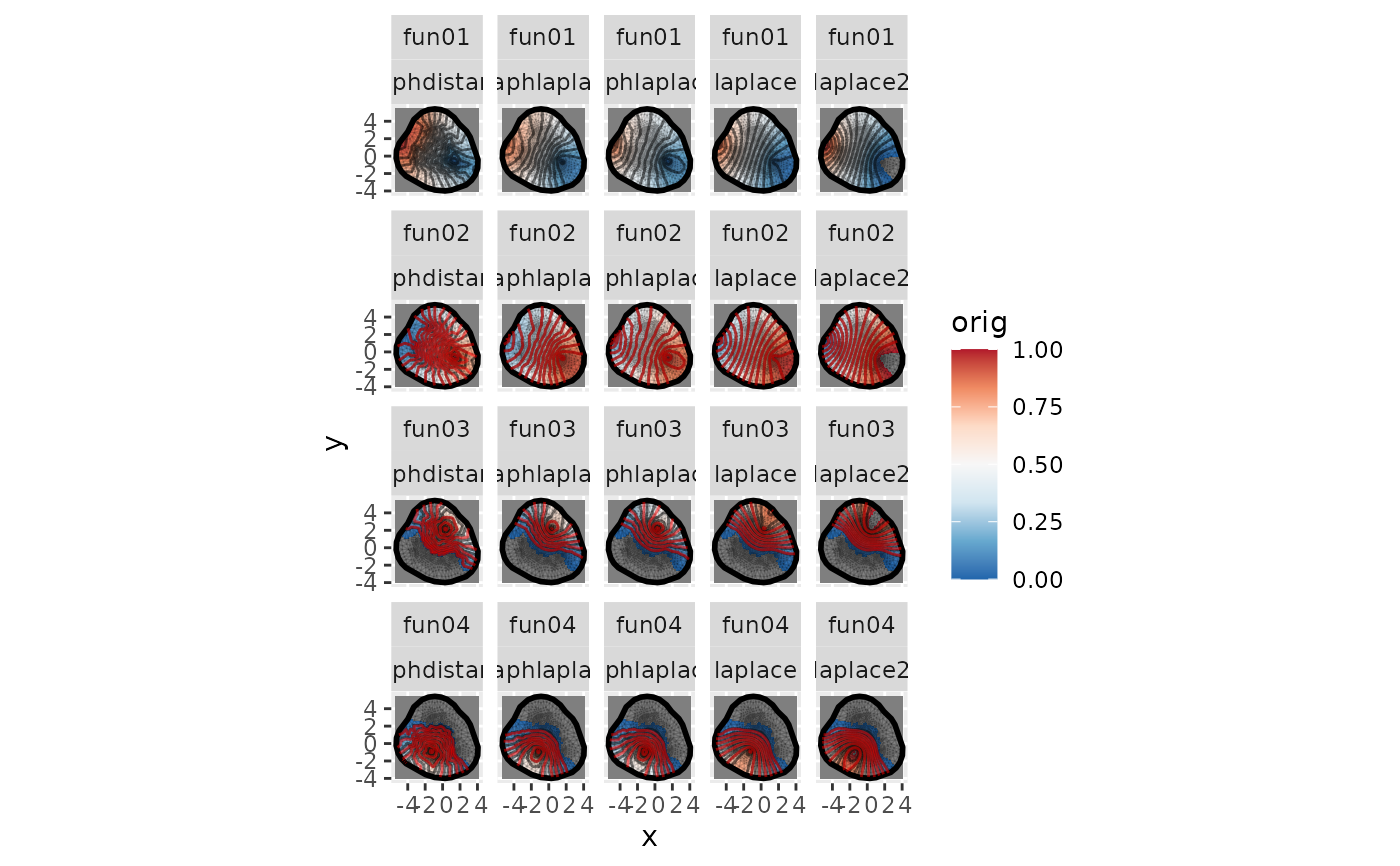
  print(
    ggplot(data = df[df$index <= 4, ]) +
      geom_tile(aes(x, y, fill = orig),
        na.rm = TRUE
      ) +
      geom_fm(data = m, color = ggplot2::alpha("black", 0.1), alpha = 0) +
      geom_contour(aes(x, y, z = orig),
        breaks = seq_len(29 - 15) / (30 - 15), #* 2-0.5,
        na.rm = TRUE, col = "black", alpha = 0.5
      ) +
      geom_contour(aes(x, y, z = norm),
        breaks = seq_len(29 - 15) / (30 - 15), #* 2-0.5,
        na.rm = TRUE, col = "red", alpha = 0.5
      ) +
      scale_fill_distiller(palette = "RdBu", limits = c(0, 1)) + #* 2-0.5) +
      facet_wrap(vars(fun, method))
  )
}



# }