Observation model construction for usage with bru()

Observation model construction for usage with bru()

Usage

bru_like(
  formula = . ~ .,
  family = "gaussian",
  data = NULL,
  response_data = NULL,
  E = NULL,
  Ntrials = NULL,
  weights = NULL,
  scale = NULL,
  domain = NULL,
  samplers = NULL,
  ips = NULL,
  include = NULL,
  exclude = NULL,
  include_latent = NULL,
  used = NULL,
  allow_combine = NULL,
  control.family = NULL,
  tag = NULL,
  options = list(),
  .envir = parent.frame()
)

like(
  formula = . ~ .,
  family = "gaussian",
  data = NULL,
  response_data = NULL,
  E = NULL,
  Ntrials = NULL,
  weights = NULL,
  scale = NULL,
  domain = NULL,
  samplers = NULL,
  ips = NULL,
  include = NULL,
  exclude = NULL,
  include_latent = NULL,
  used = NULL,
  allow_combine = NULL,
  control.family = NULL,
  tag = NULL,
  options = list(),
  .envir = parent.frame()
)

bru_like_list(...)

# S3 method for class 'list'
bru_like_list(object, envir = NULL, ...)

# S3 method for class 'bru_like'
bru_like_list(..., envir = NULL)

# S3 method for class 'bru_like'
c(..., envir = NULL)

# S3 method for class 'bru_like_list'
c(..., envir = NULL)

# S3 method for class 'bru_like_list'
x[i]

Arguments

formula

a formula where the right hand side is a general R expression defines the predictor used in the model.

family

A string identifying a valid INLA::inla likelihood family. The default is gaussian with identity link. In addition to the likelihoods provided by inla (see names(INLA::inla.models()$likelihood)) inlabru supports fitting latent Gaussian Cox processes via family = "cp". As an alternative to bru(), the lgcp() function provides a convenient interface to fitting Cox processes.

data

Likelihood-specific data, as a data.frame or SpatialPoints[DataFrame] object.

response_data

Likelihood-specific data for models that need different size/format for inputs and response variables, as a data.frame or SpatialPoints[DataFrame] object.

E

Exposure parameter for family = 'poisson' passed on to INLA::inla. Special case if family is 'cp': rescale all integration weights by a scalar E. For sampler specific reweighting/effort, use a weight column in the samplers object, see fmesher::fm_int(). Default taken from options$E, normally 1.

Ntrials

A vector containing the number of trials for the 'binomial' likelihood. Default taken from options$Ntrials, normally 1.

weights

Fixed (optional) weights parameters of the likelihood, so the log-likelihood[i] is changed into weights[i] * log_likelihood[i]. Default value is 1. WARNING: The normalizing constant for the likelihood is NOT recomputed, so ALL marginals (and the marginal likelihood) must be interpreted with great care.

scale

Fixed (optional) scale parameters of the precision for several models, such as Gaussian and student-t response models.

domain, samplers, ips

Arguments used for family="cp".

domain: Named list of domain definitions.
samplers: Integration subdomain for 'cp' family.
ips: Integration points for 'cp' family. Defaults to fmesher::fm_int(domain, samplers). If explicitly given, overrides domain and samplers.

include, exclude, include_latent

Arguments controlling what components and effects are available for use in the predictor expression.

include: Character vector of component labels that are used as effects by the predictor expression; If NULL (default), the bru_used() method is used to extract the variable names from the formula.
exclude: Character vector of component labels to be excluded from the effect list determined by the include argument. Default is NULL; do not remove any components from the inclusion list.
include_latent: Character vector. Specifies which latent state variables are directly available to the predictor expression, with a _latent suffix. This also makes evaluator functions with suffix _eval available, taking parameters main, group, and replicate, taking values for where to evaluate the component effect that are different than those defined in the component definition itself (see component_eval()). If NULL, the bru_used() method auto-detects use of _latent and _eval in the predictor expression.

used

Wither NULL (default) or a bru_used() object, that overrides the include, exclude, include_latent arguments. When used is NULL (default), the information about what effects and latent vectors are made available to the predictor evaluation is defined by

used <- bru_used(
  formula,
  effect = include,
  effect_exclude = exclude,
  latent = include_latent
)

allow_combine

logical; If TRUE, the predictor expression may involve several rows of the input data to influence the same row. When NULL, defaults to FALSE, unless response_data is non-NULL, or data is a list, or the likelihood construction requires it.

control.family

A optional list of INLA::control.family options

tag

character; Name that can be used to identify the relevant parts of INLA predictor vector output, via bru_index().

options

A bru_options options object or a list of options passed on to bru_options()

.envir

The evaluation environment to use for special arguments (E, Ntrials, weights, and scale) if not found in response_data or data. Defaults to the calling environment.

...

For bru_like_list.bru_like, one or more bru_like objects

object

A list of bru_like objects

envir

An optional environment for the new bru_like_list object

x

bru_like_list object from which to extract element(s)

i

indices specifying elements to extract

Value

A likelihood configuration which can be used to parameterise bru().

Methods (by generic)

bru_like_list(bru_like): Combine several bru_like likelihoods into a bru_like_list object
c(bru_like): Combine several bru_like likelihoods and/or bru_like_list objects into a bru_like_list object

Functions

like(): Legacy like() method.
bru_like_list(): Combine bru_like likelihoods into a bru_like_list object
bru_like_list(list): Combine a list of bru_like likelihoods into a bru_like_list object
c(bru_like_list): Combine several bru_like likelihoods and/or bru_like_list objects into a bru_like_list object

Author

Fabian E. Bachl bachlfab@gmail.com

Finn Lindgren finn.lindgren@gmail.com

Examples

# \donttest{
if (bru_safe_inla() &&
    require(ggplot2, quietly = TRUE)) {

  # The like function's main purpose is to set up models with multiple likelihoods.
  # The following example generates some random covariates which are observed through
  # two different random effect models with different likelihoods

  # Generate the data

  set.seed(123)

  n1 <- 200
  n2 <- 10

  x1 <- runif(n1)
  x2 <- runif(n2)
  z2 <- runif(n2)

  y1 <- rnorm(n1, mean = 2 * x1 + 3)
  y2 <- rpois(n2, lambda = exp(2 * x2 + z2 + 3))

  df1 <- data.frame(y = y1, x = x1)
  df2 <- data.frame(y = y2, x = x2, z = z2)

  # Single likelihood models and inference using bru are done via

  cmp1 <- y ~ -1 + Intercept(1) + x
  fit1 <- bru(cmp1, family = "gaussian", data = df1)
  summary(fit1)

  cmp2 <- y ~ -1 + Intercept(1) + x + z
  fit2 <- bru(cmp2, family = "poisson", data = df2)
  summary(fit2)

  # A joint model has two likelihoods, which are set up using the like function

  lik1 <- like("gaussian", formula = y ~ x + Intercept, data = df1)
  lik2 <- like("poisson", formula = y ~ x + z + Intercept, data = df2)

  # The union of effects of both models gives the components needed to run bru

  jcmp <- ~ x + z + Intercept(1)
  jfit <- bru(jcmp, lik1, lik2)

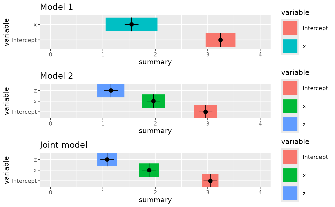
  # Compare the estimates

  p1 <- ggplot() +
    gg(fit1$summary.fixed, bar = TRUE) +
    ylim(0, 4) +
    ggtitle("Model 1")
  p2 <- ggplot() +
    gg(fit2$summary.fixed, bar = TRUE) +
    ylim(0, 4) +
    ggtitle("Model 2")
  pj <- ggplot() +
    gg(jfit$summary.fixed, bar = TRUE) +
    ylim(0, 4) +
    ggtitle("Joint model")

  multiplot(p1, p2, pj)
}

# }

Observation model construction for usage with `bru()`