The goal of inlabru is to facilitate spatial modeling using integrated nested Laplace approximation via the R-INLA package. Additionally, extends the GAM-like model class to more general nonlinear predictor expressions, and implements a log Gaussian Cox process likelihood for modeling univariate and spatial point processes based on ecological survey data. Model components are specified with general inputs and mapping methods to the latent variables, and the predictors are specified via general R expressions, with separate expressions for each observation likelihood model in multi-likelihood models. A prediction method based on fast Monte Carlo sampling allows posterior prediction of general expressions of the latent variables. See Fabian E. Bachl, Finn Lindgren, David L. Borchers, and Janine B. Illian (2019), inlabru: an R package for Bayesian spatial modelling from ecological survey data, Methods in Ecology and Evolution, British Ecological Society, 10, 760–766, doi:10.1111/2041-210X.13168, and citation("inlabru").
The inlabru.org website has links to old tutorials with code examples for versions up to 2.1.13. For later versions, updated versions of these tutorials, as well as new examples, can be found at https://inlabru-org.github.io/inlabru/articles/
Installation
You can install the current CRAN version version of inlabru, using the basic install.packages() function, or pak, after adding the INLA repository added to the list of repositories:
options(repos = c(
  INLA = "https://inla.r-inla-download.org/R/testing",
  getOption("repos")
))
install.packages("inlabru")
or
# install.packages("pak")
pak::pak("inlabru")
Development version on r-universe
Track the development version builds via inlabru-org.r-universe.dev:
options(repos = c(
  inlabruorg = "https://inlabru-org.r-universe.dev",
  getOption("repos")
))
pak::pak("inlabru")
This will pick the r-universe version if it is more recent than the CRAN version.
Example
This is a basic example which shows how fit a simple spatial Log Gaussian Cox Process (LGCP) and predicts its intensity:
# Load libraries
library(INLA)
#> Loading required package: Matrix
#>
library(inlabru)
library(fmesher)
library(ggplot2)

# Construct latent model components
matern <- inla.spde2.pcmatern(
  gorillas_sf$mesh,
  prior.sigma = c(0.1, 0.01),
  prior.range = c(0.01, 0.01)
)
cmp <- ~ mySmooth(geometry, model = matern) + Intercept(1)
# Fit LGCP model
# This particular bru/bru_obs combination has a shortcut function lgcp() as well
fit <- bru(
  cmp,
  bru_obs(
    formula = geometry ~ .,
    family = "cp",
    data = gorillas_sf$nests,
    samplers = gorillas_sf$boundary,
    domain = list(geometry = gorillas_sf$mesh)
  ),
  options = list(control.inla = list(int.strategy = "eb"))
)

# Predict Gorilla nest intensity
lambda <- predict(
  fit,
  fm_pixels(gorillas_sf$mesh, mask = gorillas_sf$boundary),
  ~ exp(mySmooth + Intercept)
)
# Plot the result
ggplot() +
  geom_fm(data = gorillas_sf$mesh) +
  gg(lambda, geom = "tile") +
  gg(gorillas_sf$nests, color = "red", size = 0.5, alpha = 0.5) +
  ggtitle("Nest intensity per km squared") +
  xlab("") +
  ylab("")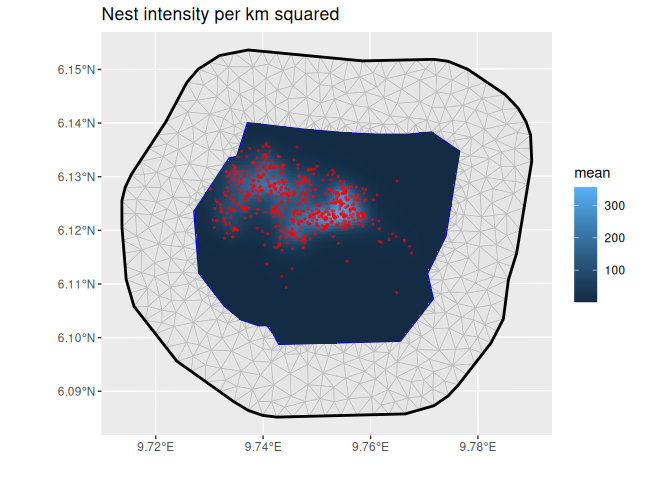
Nest intensity per km squared