SPDE models on 3D meshes • inlamesh3d

The inlamesh3d package is a temporary add-on package for INLA to test new code for using tetrahedralisation meshes for 3D SPDE models. Load INLA first, so that the new methods provided by inlamesh3d take precedence:

library(INLA)
#> Loading required package: Matrix
#> Loading required package: sp
#> This is INLA_24.06.27 built 2024-06-27 02:36:04 UTC.
#>  - See www.r-inla.org/contact-us for how to get help.
#>  - List available models/likelihoods/etc with inla.list.models()
#>  - Use inla.doc(<NAME>) to access documentation
library(inlamesh3d)
#> Loading required package: fmesher
#> 
#> Attaching package: 'inlamesh3d'
#> The following objects are masked from 'package:INLA':
#> 
#>     inla.spde2.matern, inla.spde2.pcmatern

A simple test case

To test the basic features, we construct a mesh with a single tetrahedron:

mesh <- inla.mesh3d(
  rbind(
    c(0, 0, 0),
    c(1, 0, 0),
    c(0, 1, 0),
    c(0, 0, 1)
  ),
  rbind(c(1, 2, 3, 4))
)

The finite element structure matrices can be obtained in the same way as for the traditional 2D triangle meshes:

fem <- fm_fem(mesh)

We can extract the matrices to construct a precision matrix manually, for $(1-\nabla\cdot\nabla)u(s)=\dot{W}(s)$ :

Q <- with(fem, c0 + 2 * g1 + g2)
solve(Q)
#> 4 x 4 sparse Matrix of class "dgCMatrix"
#>                                         
#> [1,] 6.062284 5.979239 5.979239 5.979239
#> [2,] 5.979239 6.646920 5.686920 5.686920
#> [3,] 5.979239 5.686920 6.646920 5.686920
#> [4,] 5.979239 5.686920 5.686920 6.646920

On a larger 3D domain, this model has an exponential covariance function, but with just a single tetrahedron, and Neumann boundary conditions, we should not expect to see this in this test case.

The new param2.matern method is used to construct the covariance parameter prior distribution model, which is then used by the new version of inla.spde2.matern:

spde <- inlamesh3d::inla.spde2.matern(
  mesh,
  param = param2.matern(mesh,
    alpha = 2,
    prior_range = 0.1,
    prior_sigma = 1
  )
)

The internal parameterisation used by param2.matern is different to the old param2.matern.orig parameterisation, and is more similar to the one used by inla.spde2.pcmatern, in that the user-visible aspects are range and standard deviation instead of $\tau$ and $\kappa$ .

Mapping data locations works the same as before. Here we verify that mapping the mesh vertices themselves produces an identity matrix:

A <- inla.spde.make.A(mesh, mesh$loc)
#> Handling: #T = 1, #loc = 4, #loc/#T = 4
#> Handled: Time/(10^3 Tetra) = 3
A
#> 4 x 4 sparse Matrix of class "dgCMatrix"
#>             
#> [1,] 1 0 0 0
#> [2,] 0 1 0 0
#> [3,] 0 0 1 0
#> [4,] 0 0 0 1

Estimation example

mesh_n <- 1000
mesh_loc <- matrix(rnorm(mesh_n * 3), mesh_n, 3)
tetra <- geometry::delaunayn(mesh_loc)
mesh <- inla.mesh3d(loc = mesh_loc, tv = tetra)
range0 <- 1 # Prior median range
sigma0 <- 1 # Prior median standard deviation
spde <- inlamesh3d::inla.spde2.matern(
  mesh,
  param = param2.matern(mesh,
    alpha = 2,
    prior_range = range0,
    prior_sigma = sigma0
  )
)

The parameterisation is in log-range and log-sigma relative to the prior medians, so that theta = log(c(range, sigma) / c(range0, sigma0)) is used to specify the internal parameter vector:

Q <- inla.spde2.precision(spde, theta = log(c(1.5, 2) / c(range0, sigma0)))
A0 <- inla.spde.make.A(mesh, cbind(0, 0, 0))
#> Splitting 1 into L: #T = 3196 #loc = 1
#> Splitting 2 into L: #T = 1598 #loc = 1
#> Splitting 3 into L: #T = 799 #loc = 1
#> Handling: #T = 799, #loc = 1, #loc/#T = 0.00125156445556946
#> Handled: Time/(10^3 Tetra) = 0.0626
#> Splitting 3 into R: #T = 799 #loc = 1
#> Handling: #T = 799, #loc = 1, #loc/#T = 0.00125156445556946
#> Handled: Time/(10^3 Tetra) = 0.0663
#> Splitting 2 into R: #T = 1598 #loc = 1
#> Splitting 3 into L: #T = 799 #loc = 1
#> Handling: #T = 799, #loc = 1, #loc/#T = 0.00125156445556946
#> Handled: Time/(10^3 Tetra) = 0.0626
#> Splitting 3 into R: #T = 799 #loc = 1
#> Handling: #T = 799, #loc = 1, #loc/#T = 0.00125156445556946
#> Handled: Time/(10^3 Tetra) = 0.0626
#> Splitting 1 into R: #T = 3196 #loc = 1
#> Splitting 2 into L: #T = 1598 #loc = 1
#> Splitting 3 into L: #T = 799 #loc = 1
#> Handling: #T = 799, #loc = 1, #loc/#T = 0.00125156445556946
#> Handled: Time/(10^3 Tetra) = 0.0663
#> Splitting 3 into R: #T = 799 #loc = 1
#> Handling: #T = 799, #loc = 1, #loc/#T = 0.00125156445556946
#> Handled: Time/(10^3 Tetra) = 0.0626
#> Splitting 2 into R: #T = 1598 #loc = 1
#> Splitting 3 into L: #T = 799 #loc = 1
#> Handling: #T = 799, #loc = 1, #loc/#T = 0.00125156445556946
#> Handled: Time/(10^3 Tetra) = 0.0626
#> Splitting 3 into R: #T = 799 #loc = 1
#> Handling: #T = 799, #loc = 1, #loc/#T = 0.00125156445556946
#> Handled: Time/(10^3 Tetra) = 0.0676
D0 <- rowSums(mesh$loc^2)^0.5

ggplot2::ggplot(data.frame(
  dist = D0,
  covariance = as.vector(solve(Q, t(A0))),
  exponential = 2^2 * exp(-D0 * (sqrt(8 * 0.5) / 1.5))
)) +
  ggplot2::geom_point(ggplot2::aes(dist, covariance)) +
  ggplot2::geom_line(ggplot2::aes(dist, exponential), col = "red")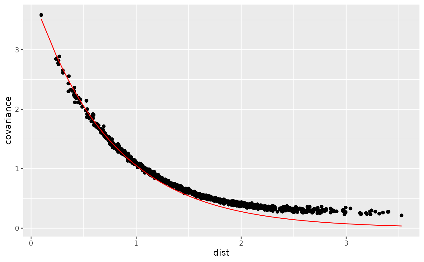

Spatial covariance function. A solid curve shows the theoretical covariance. Points show the numerical approximation covariance.

We can see some boundary effect due to the finite domain but overall the covariances follow the theory.

Let’s simulate a field and observe at some locations (here chosen as a subset of the mesh points):

x <- inla.qsample(1, Q)[, 1]
loc <- mesh$loc[seq_len(100), , drop = FALSE]
Aobs <- inla.spde.make.A(mesh, loc)
#> Splitting 1 into L: #T = 3196 #loc = 93
#> Splitting 2 into L: #T = 1598 #loc = 87
#> Splitting 3 into L: #T = 799 #loc = 70
#> Handling: #T = 799, #loc = 70, #loc/#T = 0.0876095118898623
#> Handled: Time/(10^3 Tetra) = 0.602
#> Splitting 3 into R: #T = 799 #loc = 85
#> Handling: #T = 799, #loc = 85, #loc/#T = 0.106382978723404
#> Handled: Time/(10^3 Tetra) = 0.718
#> Splitting 2 into R: #T = 1598 #loc = 68
#> Splitting 3 into L: #T = 799 #loc = 51
#> Handling: #T = 799, #loc = 51, #loc/#T = 0.0638297872340425
#> Handled: Time/(10^3 Tetra) = 0.494
#> Splitting 3 into R: #T = 799 #loc = 58
#> Handling: #T = 799, #loc = 58, #loc/#T = 0.0725907384230288
#> Handled: Time/(10^3 Tetra) = 0.507
#> Splitting 1 into R: #T = 3196 #loc = 98
#> Splitting 2 into L: #T = 1598 #loc = 91
#> Splitting 3 into L: #T = 799 #loc = 73
#> Handling: #T = 799, #loc = 73, #loc/#T = 0.0913642052565707
#> Handled: Time/(10^3 Tetra) = 0.598
#> Splitting 3 into R: #T = 799 #loc = 64
#> Handling: #T = 799, #loc = 64, #loc/#T = 0.0801001251564456
#> Handled: Time/(10^3 Tetra) = 0.487
#> Splitting 2 into R: #T = 1598 #loc = 91
#> Splitting 3 into L: #T = 799 #loc = 76
#> Handling: #T = 799, #loc = 76, #loc/#T = 0.0951188986232791
#> Handled: Time/(10^3 Tetra) = 0.583
#> Splitting 3 into R: #T = 799 #loc = 65
#> Handling: #T = 799, #loc = 65, #loc/#T = 0.081351689612015
#> Handled: Time/(10^3 Tetra) = 0.541
data <- data.frame(y = as.vector(Aobs %*% x) + rnorm(nrow(loc), sd = 0.1))

stk <- inla.stack(
  data = list(y = data$y),
  A = list(Aobs),
  effects = list(inla.spde.make.index("field", spde$n.spde))
)
est <- inla(y ~ -1 + f(field, model = spde),
  data = inla.stack.data(stk, spde = spde),
  control.predictor = list(A = inla.stack.A(stk)),
  verbose = FALSE
)

Extracting the parameter estimates and transforming them to user-interpretable scale:

quant <- c("0.025quant", "0.5quant", "0.975quant")
param_estimates <- rbind(
  range = exp(est$summary.hyperpar["Theta1 for field", quant]) * range0,
  sigma = exp(est$summary.hyperpar["Theta2 for field", quant]) * sigma0,
  obs_sigma = as.vector(as.matrix(
    est$summary.hyperpar["Precision for the Gaussian observations", rev(quant)]^-0.5
  ))
)

	0.025quant	0.5quant	0.975quant
range	1.010920	1.4169519	2.0639256
sigma	1.695369	1.9564373	2.2723690
obs_sigma	0.003378	0.0084443	0.0289314

The observation noise standard deviation is underestimated (true value was $0.1$ ), but the range and sigma parameters recover the true values, $1.5$ and $2$ , respectively.

Plotting

Experimental code:

plot(mesh)

locgrid <- as.matrix(expand.grid(1:10, 1:11, 1:12)) + rnorm(10 * 11 * 12, sd = 1e-6)
meshgrid <- inla.mesh3d(locgrid, geometry::delaunayn(locgrid))
plot(meshgrid,
  include = c(0.5, 0.5, 1),
  alpha = c(0.5, 0.5, 0.9),
  fill_col = inla.generate.colors(meshgrid$loc)$colors
)
rgl::clipplanes3d(rbind(c(1, 0, 0), c(0, 1, 0), c(0, 0, 1)), d = 0)

PC prior

Using a PC prior implementation. For illustration purposes, we use priors with the true parameter values as prior medians for the spatial range (range) and field standard deviation (sigma).

spde2 <- inlamesh3d::inla.spde2.pcmatern(
  mesh,
  alpha = 2,
  prior.range = c(range0, 0.5),
  prior.sigma = c(sigma0, 0.5)
)
est2 <- inla(y ~ -1 + f(field, model = spde2),
  data = inla.stack.data(stk, spde2 = spde2),
  control.predictor = list(A = inla.stack.A(stk)),
  verbose = FALSE
)
param_estimates2 <- rbind(
  range = est2$summary.hyperpar["Range for field", quant],
  sigma = est2$summary.hyperpar["Stdev for field", quant],
  obs_sigma = as.vector(as.matrix(
    est2$summary.hyperpar["Precision for the Gaussian observations", rev(quant)]^-0.5
  ))
)

	0.025quant	0.5quant	0.975quant
range	1.0026529	1.420249	2.0928056
sigma	1.7026729	1.967145	2.2897465
obs_sigma	0.0032848	0.008558	0.0302939